19  High-resolution phenology

Packages

library(terra)
library(ggplot2)
library(tidyr)
library(lubridate) # dates and times handling
library(mapview) # live maps
library(minpack.lm) # nonlinear fit based on a more robust optimization
# mapviewOptions(fgb = FALSE)

Dates and time

The basic R installation provides a class and functions to deal with dates and times. The as.Date() function converts a character string into a Date object. By default, the date string must be formatted either as "%Y-%m-%d" or as "%Y/%m/%d", where %Y, %m, and %d denote 4-digit year, 2-digit month and day, respectively. See the help for ?strptime for available format codes. The function strptime() is useful if you use combined date and time information. But for our purposes as.Date() works like a charm.

when <- as.Date("2012-04-21")
class(when)

[1] "Date"

Subtracting two Date objects returns a difftime object.

t1 <- as.Date("2022-04-21")
t2 <- as.Date("2022-09-13")
elapsed_time <- t2 - t1
class(elapsed_time)

[1] "difftime"

elapsed_time

Time difference of 145 days

By default a suitable unit is chosen (days). If you want a different unit, you can call the difftime() function directly. Note that units = “days” means a period of 24 hours, hence takes no account of Daylight Savings Time.

difftime(t1, t2, unit='weeks')

Time difference of -20.71429 weeks

Limited arithmetic is available on difftime objects: they can be added or subtracted, and multiplied or divided by a numeric vector.

elapsed_time * 2

Time difference of 290 days

You can convert the difftime object to a numeric vector, specifying the units you want.

as.double(elapsed_time, units="days")

[1] 145

as.double(elapsed_time, units="weeks")

[1] 20.71429

The lubridate package provides functions to easily access and manipulate dates and times. For example, we can extract the year, month, and day:

year(t1)

[1] 2022

month(t1)

[1] 4

day(t1) # day of month

[1] 21

yday(t1) # day of year

[1] 111

Land cover

We have a Sentinel-2 based land cover map available for the study region. We can use the map as an orientation and to explore how phenology varies by land cover.

lacov <- rast("data/pheno/X0070_Y0040_subset_landcover.tif")

lacol <- c("#FF0000", "#FFFF00", "#FFFF00", "#00C700", "#006363", "#008A00",
           "#FF6300", "#C7C763", "#C7C7C7", "#0000FF", "#C700C7", "#FFFFFF")
                      
classes = c('artificial land', 'cropland', 'cropland perennial', 
            'forest broadleaved', 'forest coniferous', 'forest mixed', 
            'shrubland', 'grassland', 'bareland', 'water', 'wetland', 
            'snow-ince')
plot(lacov, type='classes', col=lacol, levels=classes)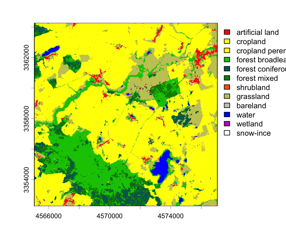

Sentinel-2

Since 2018, high-resolution phenological analyses have become possible with the Sentinel-2A/B constellation. Sentinel-2 revisits the same location on Earth 10 days at the equator with one satellite and 5 days with 2 satellites. At mid-latitudes, Sentinel-2 makes land surface observations every 2-3 days assuming cloud-free conditions. We are going to use a stack of 67 NDVI images derived from Sentinel-2 images acquired in the year 2018.

ndvi <- rast("data/pheno/X0070_Y0040_subset_s2_ndvi_2018.tif")
ndvi

class       : SpatRaster 
size        : 1200, 1200, 67  (nrow, ncol, nlyr)
resolution  : 10, 10  (x, y)
extent      : 4565056, 4577056, 3352270, 3364270  (xmin, xmax, ymin, ymax)
coord. ref. : ETRS89-extended / LAEA Europe (EPSG:3035) 
source      : X0070_Y0040_subset_s2_ndvi_2018.tif 
names       : 20180~SEN2A, 20180~SEN2A, 20180~SEN2B, 20180~SEN2B, 20180~SEN2B, 20180~SEN2B, ... 
min values  :      -10000,        -182,       -9267,       -4280,      -10000,         264, ... 
max values  :       10000,       10000,       10000,        8404,        9736,        2378, ... 

The plot window below shows an NDVI image from 7 August 2018. The NDVI values have been scaled by 10,000.

plot(ndvi["20180807_SEN2A"])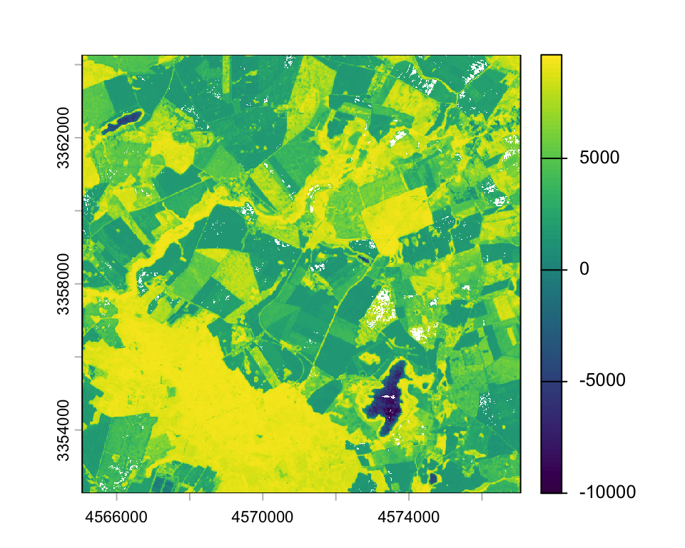

The package mapview provides great interactive plotting functionality. I do not show the plot here, due to a bug that increases the storage of this website. But you can try the code below yourself. Note, I convert the SpatRaster to an object from the older raster package, since mapview does not recognize terra objects, yet.

mapview(raster::raster(ndvi["20180807_SEN2A"]), 
                       map.types=c('Esri.WorldImagery', 'OpenStreetMap'),
                       layer.name = 'NDVI', na.color = "transparent")

Time stamps

To do time series analysis, we need date information. The dates are stored in the layer names, i.e., between 1st and 8th character.

head(names(ndvi), 5)

[1] "20180201_SEN2A" "20180208_SEN2A" "20180213_SEN2B" "20180216_SEN2B"
[5] "20180223_SEN2B"

We can extract the dates from the layer names using the function substr().

substr("20180201_SEN2A", 1, 8)

[1] "20180201"

..and convert the date string to a Date vector with as.Date().

dates <- as.Date(substr(names(ndvi), 1, 8), format='%Y%m%d')
head(dates)

[1] "2018-02-01" "2018-02-08" "2018-02-13" "2018-02-16" "2018-02-23"
[6] "2018-02-26"

The day of year (doy) will work fine as time stamp for the analysis, since we are dealing only with a single year of data.

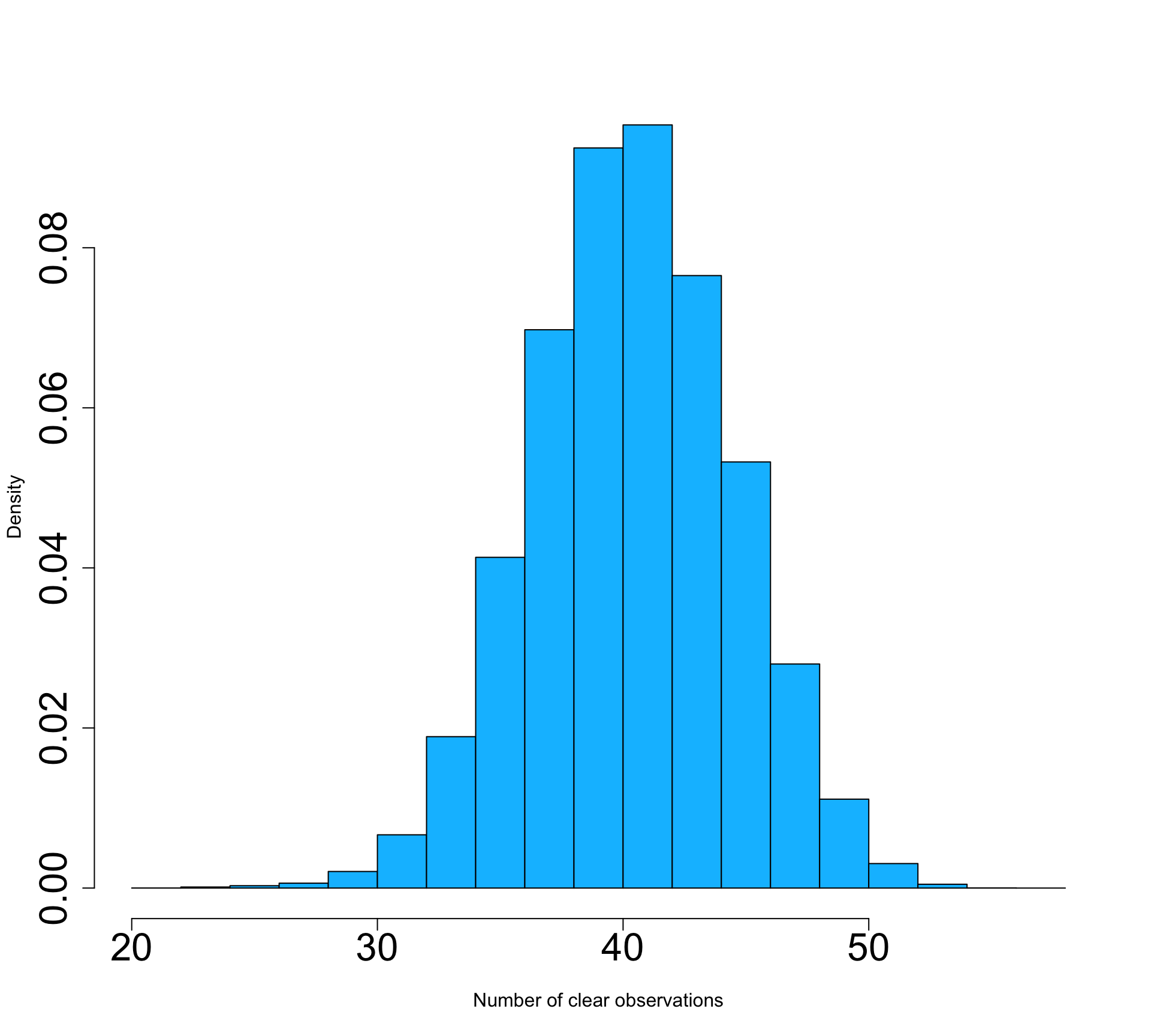
doys <- lubridate::yday(dates)

Clear observations

Data density and availability can influence the quality of time series significantly. Thus, it is a good idea to visualize the number of clear-sky observations per pixel in the NDVI deck. Clouds and shadows have been already masked out. So, we can simply count the number of observations that ar not NA. With !is.na(ndvi), we can create a binary raster stack, where TRUE indicates clear-sky observations. Note, the ! means not, in this case not NA. We can then sum up all TRUE observations for each pixel. The result is a raster, showing the number of clear observations. The number of clear observations range from 21 to 57 in 2018 in our study area. The average clear-observation count per pixel was 40.9 with a standard deviation of 4.1 observations.

n_clear <- sum(!is.na(ndvi))
plot(n_clear, pax=list(cex.axis=1.4), plg=list(cex=2))
hist(values(n_clear), main='', freq=F, col='deepskyblue',
     xlab='Number of clear observations', cex.axis=2, cex=2)

Number of clear-sky observations

Histogram of clear-sky observation density

Pixel time series

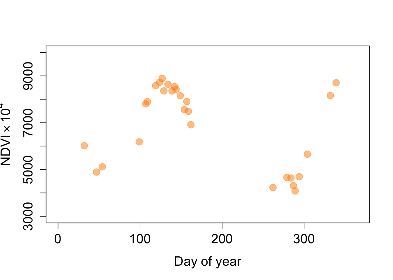
Let’s visualize the NDVI time series for a single pixel. Below, I selected one pixel over deciduous broadleaf forest (dbf) and one pixel over cropland (crop). How do these time series differ? Try selecting pixels yourself using the click() function.

pt1_dbf <- cbind(4568207, 3355387)
pt1_ndvi <- as.numeric(terra::extract(ndvi, pt1_dbf))
plot(doys, pt1_ndvi, pch=19, col=alpha('darkgreen', 0.5), cex=1.6,
     xlim=c(0, 365), ylim=c(3000, 10000), cex.axis=1.4, cex.lab=1.4,
     xlab='Day of year', ylab=expression('NDVI' %*% 10^4))
pt2_crop <- cbind(4572012, 3355967)
pt2_ndvi <- as.numeric(terra::extract(ndvi, pt2_crop))
plot(doys, pt2_ndvi, pch=19, col=alpha('darkorange', 0.5), cex=1.6,
     xlim=c(0, 365), ylim=c(3000, 10000), cex.axis=1.4, cex.lab=1.4,
     xlab='Day of year', ylab=expression('NDVI' %*% 10^4))

Sentinel-2 NDVI for a broadleaf forest pixel

Sentinel-2 NDVI for a cropland pixel

Filter

We can reduce noise by smoothing the time series with a moving average filter. R has a built-in filter() function that applies a convolution or recursive filter to a univariate time series. The function is not to be confused with the filter function in the dplyr package. Here, we will apply a convolution of a weighted average filter of size 3. The kernel weights must be odd and sum to 1. To avoid too much smoothing, we use a kernel that puts more weight on the filtered observation than on its neighbors.

pt2_doy <- doys[!is.na(pt2_ndvi)] # day of years to valid NDVI
pt2_ndvi <- pt2_ndvi[!is.na(pt2_ndvi)] # remove NA from NDVI

kernel <- c(0.25, 0.5, 0.25)
ndvi_filtered <- stats::filter(pt2_ndvi, filter=kernel, method="convolution")
head(ndvi_filtered, 10)

Time Series:
Start = 1 
End = 10 
Frequency = 1 
 [1]      NA 5227.75 5325.50 6320.50 7421.50 8044.25 8447.25 8734.00 8719.25
[10] 8563.75

The filter() function returns a time series object of class ts. To add the filtered observations to a data.frame, we need to convert the ts object into a vector.

df_ndvi <- data.frame(doy=pt2_doy, ndvi=pt2_ndvi, var='NDVI')
df_filter <- data.frame(doy=pt2_doy, ndvi=as.vector(ndvi_filtered), 
                         var='Filtered')

ggplot(rbind(df_ndvi, df_filter), aes(x = doy, y = ndvi, col = var)) +
  geom_point() + theme(legend.position="bottom") + ylab('NDVI')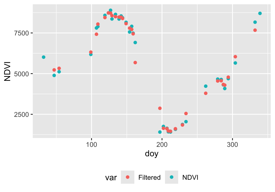

Logistic function

We noticed that croplands may not follow a typical double logistic function. If we are only interested in estimating the day of green-up (start-of-season), we can fit a single logistic function (Kowalski et al., 2020). Note, there are other alternative estimation methods that make less assumptions about the functional form, but you’ll see that the logistic function and double logistic function are quite powerful if used smartly.

\[VI(t) = wVI + \frac{mVI-wVI}{1 + e^{-mS(t-S)}} \tag{19.1}\]

Unfold the code below to see the function lgFun, which calculates NDVI based on logistic function parameters \(p\) and time \(t\).

lgFun <- function(t, p){
  result <- p["wVI"] + ((p["mVI"]-p["wVI"]) / (1 + exp(-p["mS"] * (t - p["S"]))))
  return(result)
}

Unfold the code below to see the function lgFit, which estimates the logistic function parameters based on NDVI and day of year.

lgFit <- function(t, vi, start) {
  
  # t: time
  # vi: vegetation index
  # start: start parameters
  
  wVI = min(vi)
  mVI = max(vi)

  # Define formula
  formula <- vi ~ wVI + ((mVI-wVI) / (1 + exp(-mS * (t - S))))
  
  # Fit function
  dlmodel <- tryCatch(error=function(e) NULL,
                      nlsLM(formula, start=start, na.action="na.omit"))
  
  if (is.null(dlmodel)) {
    # create parameter vector with NA's 
    # that is return in case of error
    dlcoef <- start
    dlcoef[1:length(dlcoef)] <- NA
  } else {
    # extract model coefficients
    dlcoef <- coef(dlmodel)
  }
  
  return(dlcoef)

}

When fitting the logistic model, we need to keep in mind that the NDVI values are scaled from -10000 to 10000. We could divide NDVI by 10000, but to save space and computing time, we simply adjust the parameters \(wVI\) and \(mVI\) accordingly.

params <- c(wVI=4000, mVI=9400, mS=0.2, S=114)

plot(doys, pt1_ndvi, ylim=c(3000,10000), xlim=c(0,370))
lines(1:365, lgFun(t=1:365, params))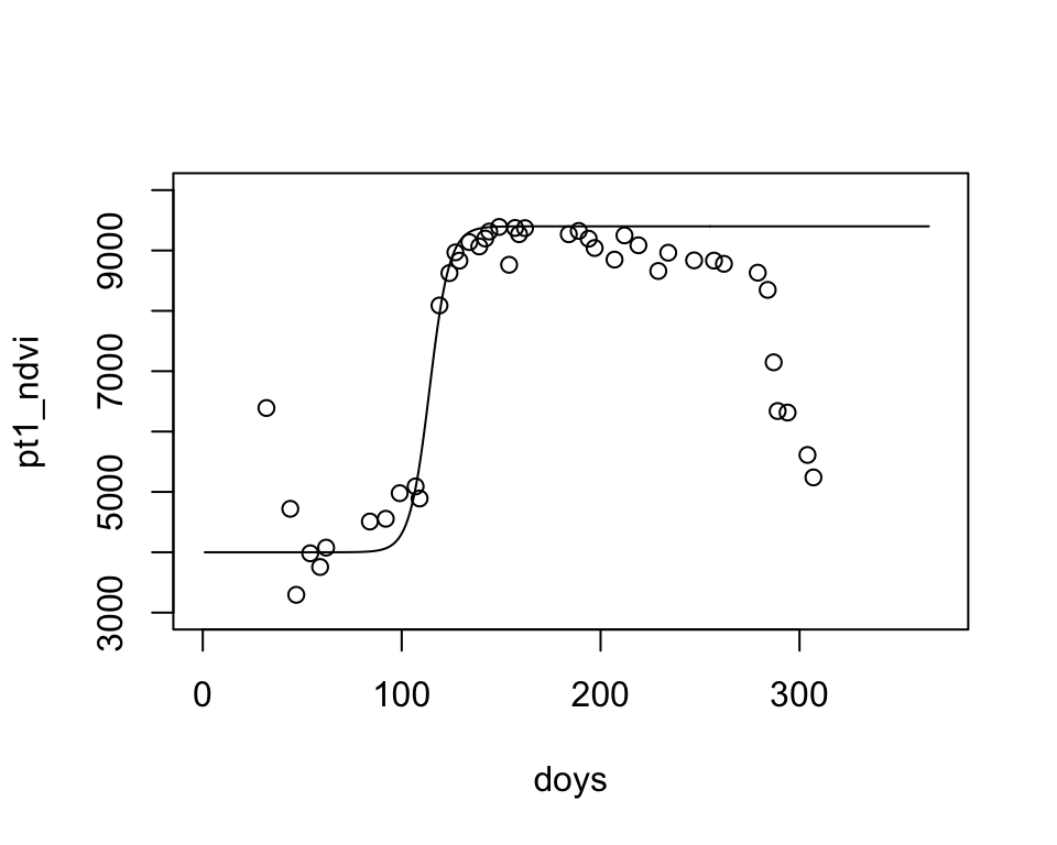

# remove NA's
t <- doys[!is.na(pt1_ndvi)]
y <- pt1_ndvi[!is.na(pt1_ndvi)]

# apply filter
yf <- stats::filter(y, filter=c(0.25, 0.5, 0.25), method="convolution")

# remove NA's from filter
t <- t[!is.na(yf)]
y <- yf[!is.na(yf)]

# We will model the logistic function from t to t_max,
# where t_max is t of the maximum NDVI plus some days buffer
t_max <- t[which.max(y)] + 10
y <- y[t < t_max]
t <- t[t < t_max]

# fit logistic model
starters <- c(wVI=4000, mVI=9400, mS=0.2, S=114)
coefs <- lgFit(t, y, starters)
coefs

         wVI          mVI           mS            S 
4202.0437717 9266.6412810    0.1670042  114.5751342 

plot(t, y, ylim=c(3000,10000), xlim=c(0,370))
lines(1:365, lgFun(t=1:365, coefs))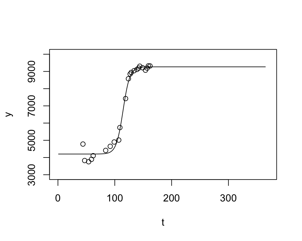

Map green-up

The function app() applies a function to the values of each cell of a SpatRaster. Below, we wrap our workflow into the function lgMap(). Note, using app() is convenient but relatively slow. The whole study area took about 30 min on my laptop. There is a multi-core option, but it may not be faster unless you have many cores and complex functions.

lgMap <- function(vi){
  
  # t: time
  # vi: vegetation index
  # start: start parameters
  
  # looks for variable doy outside the function 
  t <- doys[!is.na(vi)]
  y <- vi[!is.na(vi)]
  
  yf <- stats::filter(y, filter=c(0.25, 0.5, 0.25), method="convolution")
  
  t <- t[!is.na(yf)]
  y <- yf[!is.na(yf)]
  
  t_max <- t[which.max(y)] + 10
  y <- y[t < t_max]
  t <- t[t < t_max]
  
  starters <- c(wVI=4000, mVI=9400, mS=0.2, S=114)
  coefs <- lgFit(t, y, starters)
  
  return(coefs)
}

tictoc::tic() # measures elapsed time
phen_param <- app(ndvi, lgMap)
tictoc::toc()

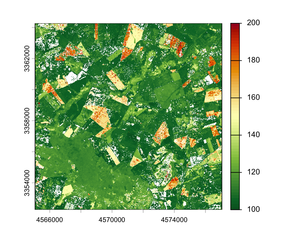
plot(phen_param$S, range=c(100, 200), col= hcl.colors(64, "RdYlGn", rev=T))

writeRaster(phen_param, "data/pheno/X0070_Y0040_subset_s2_ndvi_2018_pheno.tif")

mapview(raster::raster(phen_param$S),
                       map.types=c('Esri.WorldImagery', 'OpenStreetMap'),
                       layer.name = 'Greenup', na.color = "transparent",
                       at = seq(100, 200, 10),
                       col.regions=hcl.colors(64, "RdYlGn", rev=T))

Kowalski, K., Senf, C., Hostert, P., Pflugmacher, D., 2020. Characterizing spring phenology of temperate broadleaf forests using landsat and sentinel-2 time series. International Journal of Applied Earth Observation and Geoinformation 92. https://doi.org/10.1016/j.jag.2020.102172