library(lidR)
library(terra)15 Lidar data
Packages
We will be using the terra (Hijmans, 2024) package to process lidar raster data and the lidR package (Roussel et al., 2020; Roussel and Auty, 2022) to process lidar point (pulse) data. The lidR package also has a great online book (Roussel et al., 2022).
Lidar point data
The las format is specialized binary file format for lidar data. It can be read in R with readLAS(). The las specification document contains information on the data and metadata structure.
You can get an overview of your las file using the familiar summary()function.
las <- readLAS("data/lidar/campcreek_subset.las")summary(las)class : LAS (v1.0 format 1)
memory : 66 Mb
extent : 556716, 557113, 310826, 311222 (xmin, xmax, ymin, ymax)
coord. ref. : NA
area : 160000 units²
points : 1.3 million points
type : airborne
density : 8.3 points/units²
density : 7.5 pulses/units²
File signature: LASF
File source ID: 0
Global encoding:
- GPS Time Type: GPS Week Time
- Synthetic Return Numbers: no
- Well Know Text: CRS is GeoTIFF
- Aggregate Model: false
Project ID - GUID: 00000000-0000-0000-0000-000000000000
Version: 1.0
System identifier:
Generating software: rlas R package
File creation d/y: 0/2017
header size: 227
Offset to point data: 227
Num. var. length record: 0
Point data format: 1
Point data record length: 28
Num. of point records: 1330997
Num. of points by return: 1192740 133038 5197 22 0
Scale factor X Y Z: 0.01 0.01 0.01
Offset X Y Z: 0 0 0
min X Y Z: 556716 310826 1487
max X Y Z: 557113 311222 1625
Variable Length Records (VLR): void
Extended Variable Length Records (EVLR): voidThe las file contains the data table and header information. You can access them with @data and @header, respectively.
head(las@data, 5)| X | Y | Z | gpstime | Intensity | ReturnNumber | NumberOfReturns | ScanDirectionFlag | EdgeOfFlightline | Classification | Synthetic_flag | Keypoint_flag | Withheld_flag | ScanAngleRank | UserData | PointSourceID |
|---|---|---|---|---|---|---|---|---|---|---|---|---|---|---|---|
| 556717 | 310994 | 1527 | 505413 | 94 | 1 | 1 | 0 | 0 | 1 | FALSE | FALSE | FALSE | 10 | 0 | 0 |
| 556717 | 310995 | 1528 | 505413 | 108 | 1 | 1 | 0 | 0 | 1 | FALSE | FALSE | FALSE | 10 | 0 | 0 |
| 556717 | 310995 | 1528 | 505413 | 108 | 1 | 1 | 0 | 0 | 1 | FALSE | FALSE | FALSE | 10 | 0 | 0 |
| 556717 | 310995 | 1528 | 505413 | 14 | 1 | 1 | 0 | 0 | 1 | FALSE | FALSE | FALSE | 11 | 0 | 0 |
| 556717 | 310995 | 1528 | 505413 | 134 | 1 | 1 | 0 | 0 | 1 | FALSE | FALSE | FALSE | 11 | 0 | 0 |
Point classification
The field Classification can contain information of the land surface, e.g., whether the pulse was returned by bare ground, a building, or vegetation. The LAS specification defines several class codes to provide some consistency across LAS user’s. However, wether the codes were correctly used or used at all, depends on the people that created the LAS file.
| Value | Meaning |
|---|---|
| 0 | Created, never classified |
| 1 | Unclassified |
| 2 | Ground |
| 3 | Low Vegetation |
| 4 | Medium Vegetation |
| 5 | High Vegetation |
| 6 | Building |
| 7 | Low Point (noise) |
| 8 | Model Key-point (mass point) |
| 9 | Water |
| 10 | ... |
Exploration
Interactive 3-D point cloud viewer.
plot(las, color = "Classification")Get statistics about the pulse data, such as the number of points per class:
table(las@data$Classification)
      1       2
1162850  168147
Build a histogram of the elevation information.
hist(las@data$Z, main='')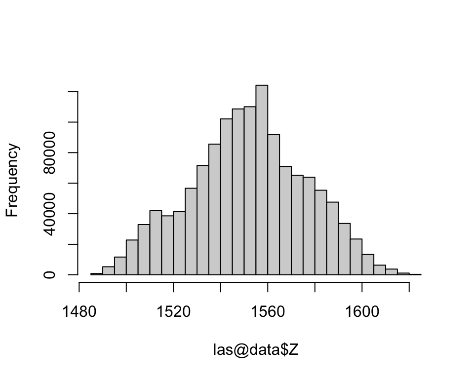
Ground identification
classify_ground() implements algorithms for segmentation of ground points. The function updates the field Classification of the LAS input object. The points classified as ‘ground’ are assigned a value of 2 in accordance with the las specifications.
ws = seq(3, 12, 3)
th = seq(0.1, 2, length.out = length(ws))
las <- classify_ground(las, algorithm=pmf(ws, th))
table(las@data$Classification)
Digital terrain model
The rasterize_terrain() functions creates a digital terrain model (SpatRaster) using a choice of algorithms, including inverse distance interpolation, krigging, triangular irregular networks (tin), a simple minimum, as well as two lidar-specific algorithms.
dtm <- rasterize_terrain(las, res=1, algorithm = knnidw(k = 8, p = 2))
plot(dtm)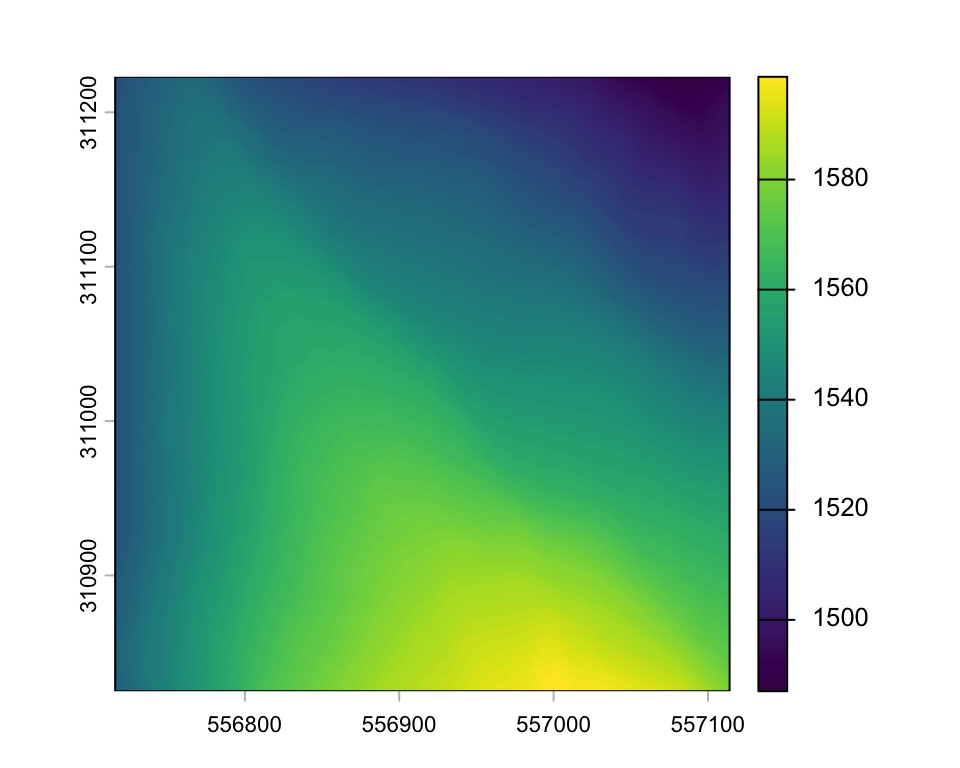
Normalization
The normalization of the lidar point data, normalizes the elevation measurements to height above ground by subtracting the digital terrain elevations (raster) from the point elevations.
lasnorm <- normalize_height(las, dtm)

# set zero values to zero
lasnorm@data$Z[lasnorm@data$Z < 0] <- 0

# write normalized point data to LAS file
# writeLAS(las, 'data/campcreek_subset_norm.las')
Visualization
plot(lasnorm)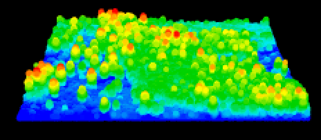
Canopy height model
We can create a raster representing the top height (or height of the hightest pulse return), also called canopy height model (CHM) or digital canopy model (DCM).
The simplest method consists of returning the highest z coordinates among all lidar returns falling into the corresponding n by n meter area (e.g. 1 x 1 m).
subset = ext(c(556990, 557095, 310870, 310965))

chm1 = rasterize_canopy(lasnorm, res = 0.5, algorithm=p2r())

chm1_zoom <- terra::crop(chm1, subset)
plot(chm1_zoom, col=height.colors(50))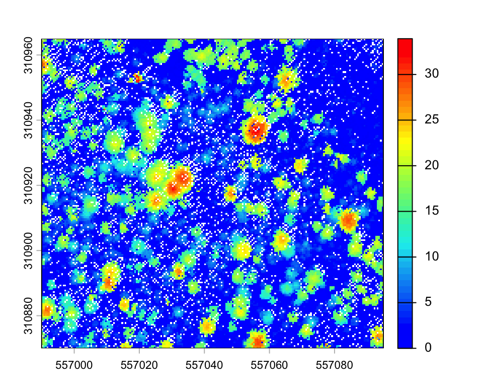
Depending on the resolution, the resulting CHM may contain empty pixels. A simple improvement can be obtained by replacing each lidar point with a small disk. Since a laser beam has a width and a footprint, this tweak may simulate this fact.
chm2 <- rasterize_canopy(lasnorm, res = 0.5, algorithm=p2r(subcircle = 0.2))

chm2_zoom <- terra::crop(chm2, subset)
plot(chm2_zoom, col=height.colors(50))
There is a trade-off between CHM resolution and disk size to avoid empty pixels. An interpolation of empty pixels can also be done with the parameter na.fill.
chm3 <- rasterize_canopy(lasnorm, res = 0.5, algorithm=p2r(subcircle = 0.2, na.fill = knnidw(k = 4, p=2)))

chm3_zoom <- terra::crop(chm3, subset)
plot(chm3_zoom, col=height.colors(50))
Pixel metrics
The function pixel_metrics computes a series of descriptive statistics defined by the user for a lidar dataset within each pixel of a raster.
hmean <- pixel_metrics(lasnorm, mean(Z), res = 10)
plot(hmean)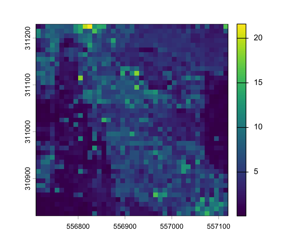
We can calculate statistics and plot the histogram of mean height.
terra::global(hmean, c("mean")) mean
V1 4.4hist(values(hmean), main='')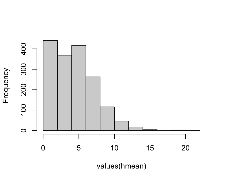
A special function to create a raster showing the point density is also available:
gdy <- rasterize_density(lasnorm, res = 10)
plot(gdy)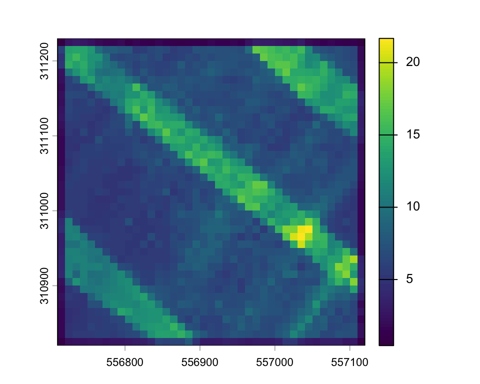
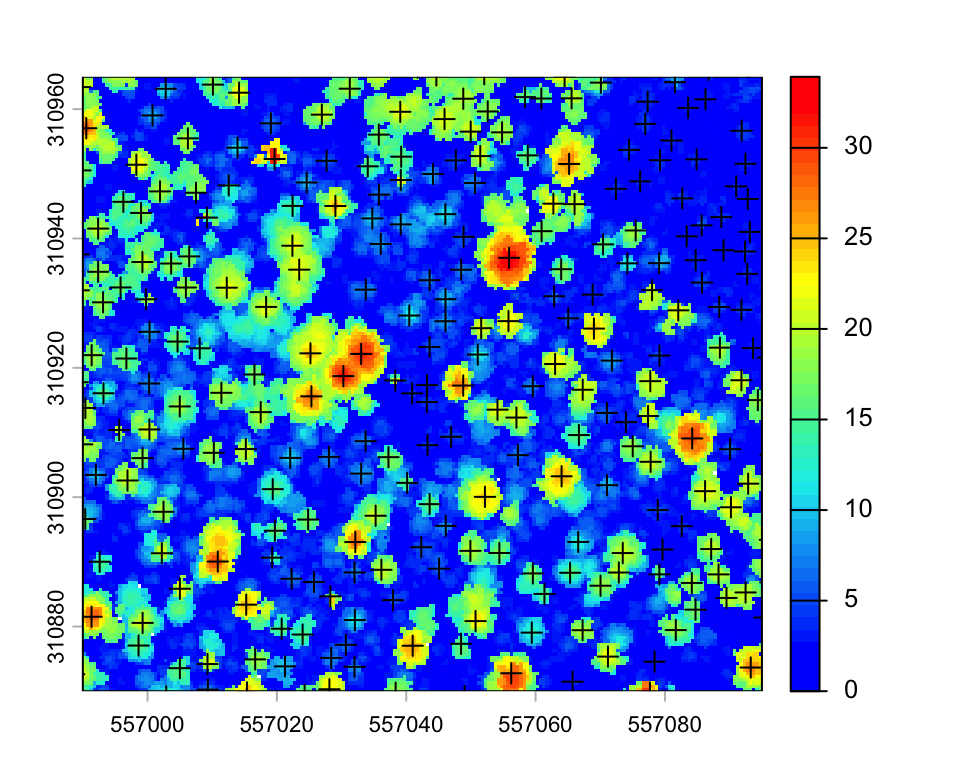
Tree detection
There are several individual tree detection and segmentation algorithms accessible through lidR. The locate_trees() function uses a maximum filter to detect tree tops. The segment_trees() function performs a segmentation, assigning unique tree id’s to each pulse return (see here).
ttops <- locate_trees(lasnorm, lmf(ws = 5))plot(chm2, col = height.colors(50), ext=subset)
plot(sf::st_geometry(ttops), add = TRUE, pch = 3)