library(terra)
library(ggplot2)10 Quantitative mapping
Packages
Background
Quantitative mapping in remote sensing involves predicting continuous variables, rather than discrete land-cover classes, using regression-based models applied to satellite imagery. This approach estimates measurable environmental parameters, such as chlorophyll concentration, vegetation biomass, or soil moisture, for every pixel across a region. By linking spectral information from satellite bands to field-measured reference data, quantitative mapping produces detailed, continuous surfaces that capture subtle spatial variations. Techniques range from simple linear regression using individual spectral bands to advanced machine learning methods like random forests or neural networks that capture complex, nonlinear patterns in multispectral or hyperspectral data.
Mapping usually involves two main steps. In the training phase, a model is built, and in the prediction phase, the trained model is applied to generate a map. Training a model requires a response variable (the quantity to be predicted) and predictor variables (the inputs used for prediction). In remote sensing, the predictor variables are derived from satellite data, while the response variable is typically obtained from field samples or interpretation of high-resolution reference data. In this chapter, we use Sentinel-2 data as predictor variables and land cover fractions derived from very high-resolution land cover maps as the response variable.

Sentinel-2
We use a Sentinel-2 image acquired over Berlin on 27 August 2016. The image was atmospherically corrected to surface reflectance using FORCE (Frantz, 2019). We can read the image using the rast function from the terra package (Chapter 6).
s2img <- terra::rast("data/frac/SEN2A_LEVEL2_BOA_20160827_berlin_clip.tif")Let’s check out the band names. In this dataset, the band names appear in double quotes "'". Let’s fix this and rename them. See here for more information on Sentinel-2 bands.
names(s2img) [1] "'B2'" "'B3'" "'B4'" "'B5'" "'B6'" "'B7'" "'B8'" "'B8A'" "'B11'"
[10] "'B12'"names(s2img) <- c('B2', 'B3', 'B4', 'B5', 'B6', 'B7', 'B8', 'B8A', 'B11', 'B12')Let’s check out the image metadata
s2imgclass : SpatRaster
size : 1450, 1702, 10 (nrow, ncol, nlyr)
resolution : 10, 10 (x, y)
extent : 385732, 402752, 5808375, 5822875 (xmin, xmax, ymin, ymax)
coord. ref. : WGS 84 / UTM zone 33N (EPSG:32633)
source : SEN2A_LEVEL2_BOA_20160827_berlin_clip.tif
names : B2, B3, B4, B5, B6, B7, ... You can use summary() to calculate image statistics. For large files, a sample is used. You can change the number of samples using size option.
summary(s2img, size=10000000) B2 B3 B4 B5
Min. :-9999.0 Min. :-9999.0 Min. :-9999.0 Min. :-9999
1st Qu.: 286.0 1st Qu.: 479.0 1st Qu.: 385.0 1st Qu.: 775
Median : 452.0 Median : 661.0 Median : 627.0 Median : 956
Mean : 563.3 Mean : 756.8 Mean : 746.3 Mean : 1022
3rd Qu.: 703.0 3rd Qu.: 890.0 3rd Qu.: 947.0 3rd Qu.: 1163
Max. :10000.0 Max. :10000.0 Max. :10000.0 Max. :10000
B6 B7 B8 B8A
Min. :-9999 Min. :-9999 Min. :-9999 Min. :-9999
1st Qu.: 1448 1st Qu.: 1602 1st Qu.: 1540 1st Qu.: 1682
Median : 1815 Median : 2080 Median : 2126 Median : 2215
Mean : 1807 Mean : 2080 Mean : 2140 Mean : 2215
3rd Qu.: 2161 3rd Qu.: 2537 3rd Qu.: 2705 3rd Qu.: 2725
Max. :10000 Max. :10000 Max. :10000 Max. :10000
B11 B12
Min. :-9999 Min. :-9999
1st Qu.: 1329 1st Qu.: 807
Median : 1512 Median : 995
Mean : 1565 Mean : 1054
3rd Qu.: 1735 3rd Qu.: 1225
Max. :10000 Max. :10000 You may notice that the band values range from –9999 to 10,000. The reflectance values, originally between 0 and 1, have been scaled by 10,000 and stored as integers to reduce file size. The value –9999 indicates missing data. We can mark these as NA and then recalculate the statistics.
NAflag(s2img) <- -9999
summary(s2img, size=10000000)
B2 B3 B4 B5
Min. : -943.0 Min. : -841.0 Min. : -495.0 Min. : -449
1st Qu.: 286.0 1st Qu.: 479.0 1st Qu.: 385.0 1st Qu.: 775
Median : 452.0 Median : 661.0 Median : 627.0 Median : 956
Mean : 563.4 Mean : 756.8 Mean : 746.3 Mean : 1022
3rd Qu.: 703.0 3rd Qu.: 890.0 3rd Qu.: 947.0 3rd Qu.: 1163
Max. :10000.0 Max. :10000.0 Max. :10000.0 Max. :10000
NA's :7 NA's :7 NA's :7 NA's :7
B6 B7 B8 B8A
Min. : -204 Min. : -396 Min. : -354 Min. : -335
1st Qu.: 1448 1st Qu.: 1602 1st Qu.: 1540 1st Qu.: 1682
Median : 1815 Median : 2080 Median : 2126 Median : 2215
Mean : 1808 Mean : 2080 Mean : 2140 Mean : 2215
3rd Qu.: 2161 3rd Qu.: 2537 3rd Qu.: 2705 3rd Qu.: 2725
Max. :10000 Max. :10000 Max. :10000 Max. :10000
NA's :7 NA's :7 NA's :7 NA's :7
B11 B12
Min. : 42 Min. : 19
1st Qu.: 1329 1st Qu.: 807
Median : 1512 Median : 995
Mean : 1565 Mean : 1054
3rd Qu.: 1735 3rd Qu.: 1225
Max. :10000 Max. :10000
NA's :7 NA's :7 Now we see that there are seven pixels with missing data. Some pixels also still have negative reflectance values. These result from slight overcompensation during the atmospheric correction process, which can overcorrect dark areas such as shadows, water, or dense vegetation, leading to small negative reflectance values.
Using the plotRGB function we can create an RGB representation of three image bands (e.g. NIR-red-green):
plotRGB(s2img, r = 7, g= 3, b = 2, stretch = "hist")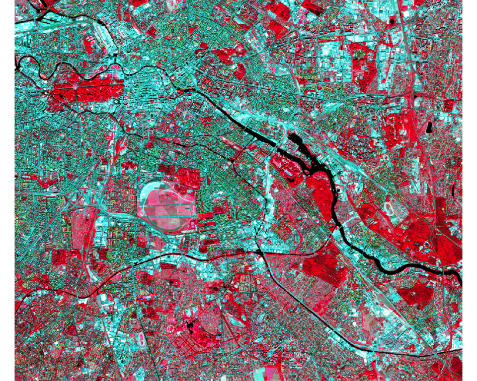
Reference data
To train a regression model, we need reference data representing land cover fractions at the Sentinel-2 pixel scale. Here, we use a high-resolution, discrete land cover map with a spatial resolution of 0.5 m × 0.5 m and aggregate it to fractions with a spatial resolution of 10 m x 10 m. The map legend includes the classes: 0 - no data, 1 - impervious surface, 2 - low vegetation < 2.5m, 3 - high vegetation, 4 - soil.
classmap <- rast("data/frac/berlin_reference_class_map.tif")
classmap
class : SpatRaster
size : 29000, 34040, 1 (nrow, ncol, nlyr)
resolution : 0.5, 0.5 (x, y)
extent : 385732, 402752, 5808375, 5822875 (xmin, xmax, ymin, ymax)
coord. ref. : WGS 84 / UTM zone 33N (EPSG:32633)
source : berlin_reference_class_map.tif
name : Band 1 plot(classmap,
type="classes",
levels=c("Impervious", "Low vegetation", "High vegetation", "Soil"))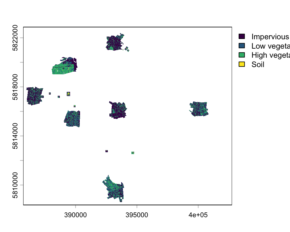
You see, the land cover map does not cover the entire area, only small patches distributed across Berlin. Let’s plot only a spatial subset:
zoom_ext <- ext(392930, 393330, 5809500, 5809855)
classmap_zoom <- crop(classmap, zoom_ext)

plot(classmap_zoom,
     type="classes", col=c("grey", "green", "darkgreen", "orange"),
     levels=c("Impervious", "Low vegetation", "High vegetation", "Soil"))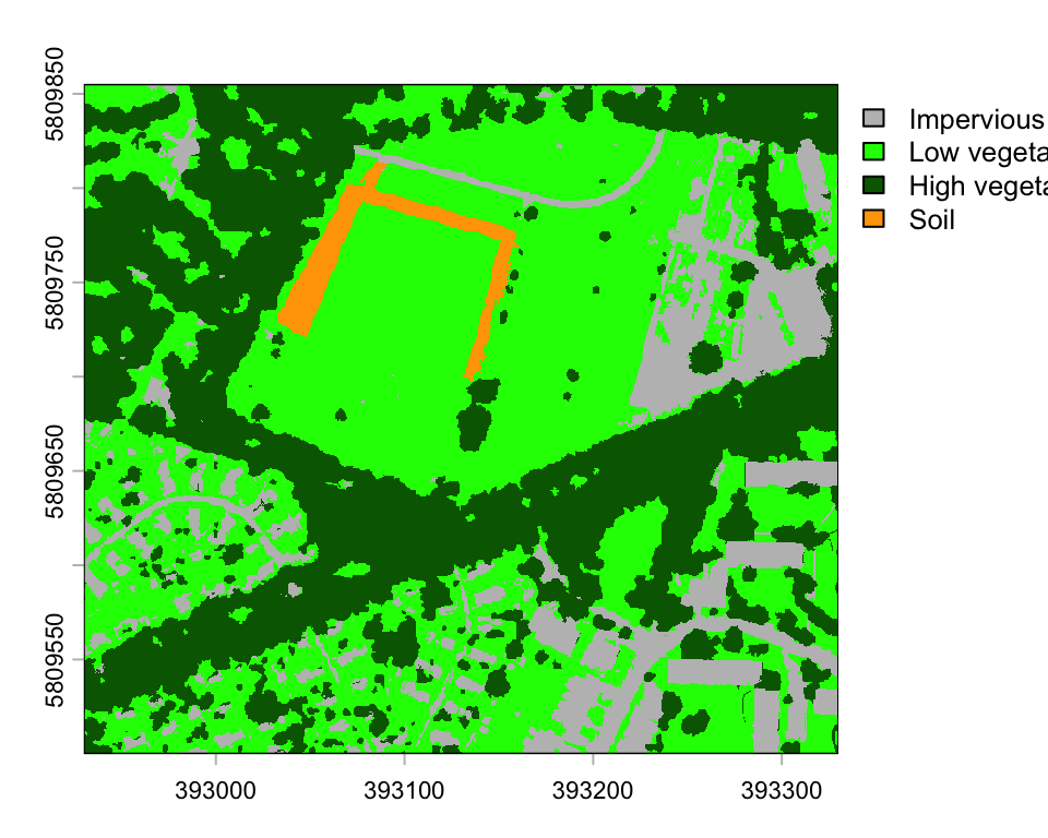
Based on this high-resolution land cover map, we can create class fractions at 10-m spatial resolution. The aggregate function from the terra package aggregates a raster to a coarser resolution determined by the aggregation factor (fact). The supplied function fun defines how the new value is calculated at the coarser resolution. For example, the fun=mean calculates the mean value of all 5 m x 5 m pixel within each 10 m x 10 m pixel.
We calculate the cover fraction for each land cover class individually. First, we generate a binary raster for the target class (e.g., classmap == 1), where pixels belonging to that class are assigned a value of TRUE, and all other pixels are assigned FALSE. In subsequent calculations, these logical values are treated numerically, with TRUE corresponding to 1 and FALSE to 0. Consequently, when we compute the mean value within each 10 m × 10 m grid cell of the binary raster, the result represents the average of a series of 0s and 1s, which is equivalent to the proportion of pixels belonging to class 1 within that cell.
# impervious fractions at 20 m x 20 m resolution
imp <- aggregate(classmap == 1, fact=20, fun=mean, na.rm=F)

# low veg fractions at 20 m x 20 m resolution
low_veg <- aggregate(classmap == 2, fact=20, fun=mean, na.rm=F)

# high veg fractions at 20 m x 20 m resolution
high_veg <- aggregate(classmap == 3, fact=20, fun=mean, na.rm=F)

# soil fractions at 20 m x 20 m resolution
soil <- aggregate(classmap == 4, fact=20, fun=mean, na.rm=F)

# stack all fraction layers into a multi-layer raster
fractionImage <- c(imp, low_veg, high_veg, soil)

# write raster to tif
writeRaster(fractionImage, filename="data/frac/berlin_reference_class_fractions.tif",
            format="GTiff", datatype="FLT4S", overwrite=T)
The resulting reference fraction images have a spatial resolution of 10 m x 10 m. We stack them together to obtain a raster with the following four layers: 1: impervious fractions, 2: low vegetation fraction, 3: high vegetation fraction, and layer 4: soil fraction.
lcf <- rast("data/frac/berlin_reference_class_fractions.tif")
names(lcf) <- c('imp', 'veglow', 'veghigh', 'soil')

# plot a subset using the ext argument
plot(lcf, ext=zoom_ext, nc=4, axes=F, cex=1.6,
     plg=list(cex=1.2), col=gray.colors(32, rev=T))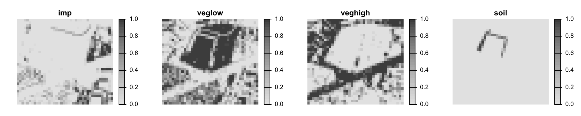
Training data
To complete our training dataset, we need to merge the reference data with Sentinel-2 data. This requires constructing a data frame that includes a sample of Sentinel-2 pixels along with their corresponding vegetation cover fractions from the reference data (also referred to as labels). Completing this step is part of your exercise. Here, we instead use an existing training dataset comprising 16 samples of NDVI values with their associated vegetation cover fractions.
train_ds <- read.csv('data/frac/NDVI_veg-ref.csv')
head(train_ds)
ndvi vegcov
1 0.85 100
2 0.78 100
3 0.81 100
4 0.85 100
5 0.77 100
6 0.67 84Simple linear regression
In this chapter, we want to use a simple linear regression model to predict land cover fractions from Sentinel-2 data. Let’s recap: a simple linear regression model is defined as follows:
\(\hat{y_i} = \beta_0 + \beta_1x_i + \epsilon_i\)
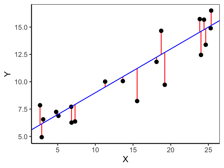
where \(y_i\) is the \(i\)’th response, \(\hat{y_i}\) is the fitted value of the \(i\)’th response, \(x_i\) the \(i\)’th predictor value, \(\beta_0\) the intercept, \(\beta_1\) the regression slope, and \(\epsilon_i\) the residual of prediction \(i\). The data pairs \(x_i\) and \(y_i\) are drawn from a sample and thus known, though we don’t know \(\beta_0\) and \(\beta_1\). We can estimate both parameters by minimizing the vertical distances \((y_i - \hat{y_i})\) (red lines in Figure 10.1) between the observed \(y_i\) (black dots in Figure 10.1) and the fitted \(\hat{y_i}\) (blue line in Figure 10.1). This technique is also called ordinary least squares (OLS) regression. Specifically, we minimize the squared distances, called the residual sum of squares (\(SS_{res}\)):
\(SS_{res} = \sum_{i=1}^{n}\epsilon_i^2 = \sum_{i=1}^{n}(y_i - \hat{y_i})^2\)
The corresponding estimator, called the Ordinary Least Squares (OLS) estimator, for a simple linear regression with one predictor is:
\(\hat{\beta_1} = \frac{\sum_{i=1}^{n}(x_i - \bar{x})(y_i - \bar{y})}{\sum_{i=1}^{n}(x_i - \bar{x})^2}\)
\(\hat{\beta_0} = \bar{y} - \hat{\beta_1}\bar{x}\)
Coefficient of determination
The coefficient of determination (\(R^2\)) is a measure of goodness-of-fit and ranges from 0 (no fit) to 1 (best fit). The closer the observations are to the regression line, the smaller the residual sum-of-squares (\(SS_{res}\)), the better does the model fit the data. If all observations lie on the regression line, then the \(R^2\) is 1, meaning there is no residual variance (\(SS_{res}\)=0). The ratio of the residual sum-of-squares (\(SS_{res}\)) to the total sum-of-squares (\(SS_{tot} = \sum_i{(y_i - \bar{y})^2}\)) is the proportion of unexplained variance. The counterpart is the proportion of explained variance. The \(R^2\) is the proportion of the variance of the response variable explained by the model:
\(R^2 = 1 - \frac{SS_{res}}{SS_{tot}}\)
The lm function
We can fit a linear model with OLS using the lm() function. The argument to lm() is a model formula in which the tilde symbol (~) should be read as described by. The names of the response variable vegcov and the predictor ndvi must match the column names in the data.frame train_ds.
vegmod <- lm(vegcov ~ ndvi, data = train_ds)The result of lm() is a model object. This is a distinctive concept of R. Whereas other statistical systems focus on generating printed output that can be controlled by setting options, you get instead the result of a model fit encapsulated in an object from which the desired quantities can be obtained using extractor functions. An lm object does in fact contain much more information than you see when it is printed.
vegmod
Call:
lm(formula = vegcov ~ ndvi, data = train_ds)

Coefficients:
(Intercept)         ndvi
      10.08       108.51
The printed output of the lm object is quite brief. It displays only the model formula and the estimated coefficients: the intercept and the slope. Together, these define the fitted regression line:
\(\hat{y} = 10.08 + 108.51x_i\)
Here, \(10.08\) is the intercept, representing the predicted value of \(y\) when \(x_i = 0\), and \(108.51\) is the slope, indicating the expected change in \(y\) for a one-unit increase in \(x_i\).
Calling summary() on an lm object provides a detailed overview of the fitted linear model. It shows the estimated coefficients with their standard errors, t-values, and p-values, allowing assessment of each predictor’s significance. It also summarizes the residuals, reports the R-squared and adjusted R-squared values to indicate how well the model explains the variability in the response, and includes the F-statistic to test the overall model fit, along with other diagnostics such as residual standard error and degrees of freedom.
summary(vegmod)
Call:
lm(formula = vegcov ~ ndvi, data = train_ds)

Residuals:
    Min      1Q  Median      3Q     Max
-15.146  -2.317   0.428   5.316  18.983

Coefficients:
            Estimate Std. Error t value Pr(>|t|)
(Intercept)   10.081      6.471   1.558    0.142
ndvi         108.514     10.226  10.611 4.46e-08 ***
---
Signif. codes:  0 '***' 0.001 '**' 0.01 '*' 0.05 '.' 0.1 ' ' 1

Residual standard error: 9.089 on 14 degrees of freedom
Multiple R-squared:  0.8894,    Adjusted R-squared:  0.8815
F-statistic: 112.6 on 1 and 14 DF,  p-value: 4.459e-08
Extractor functions
The function fitted() returns the fitted values, i.e., the y-values that you would expect for the given x-values according to the best-fitting straight line. The residuals() function shows the differences between these fitted values and the observed y-values. With predict(), you can apply the model to a new dataset to generate predicted values.
fitted(vegmod) 1 2 3 4 5 6 7 8
102.31729 94.72133 97.97674 102.31729 93.63619 82.78481 81.69968 88.21050
9 10 11 12 13 14 15 16
49.14556 29.61308 54.57124 22.01712 77.35913 77.35913 78.44427 57.82666 residuals(vegmod) 1 2 3 4 5 6
-2.3172870 5.2786745 2.0232624 -2.3172870 6.3638119 1.2151855
7 8 9 10 11 12
-13.6996772 5.7894987 -15.1455564 -14.6130839 5.4287568 18.9828776
13 14 15 16
-0.3591277 -0.3591277 -0.4442651 4.1733447 The function coefficients() returns the estimated model parameters; in this case intercept and slope.
coefficients(vegmod)(Intercept) ndvi
10.08061 108.51374 intercept <- coefficients(vegmod)[1]
slope <- coefficients(vegmod)[2]Plot fitted line
The function abline() adds a line to an existing plot. It takes a slope and intercept parameter as input. Alternatively, you can give it the model output of lm().
plot(vegcov ~ ndvi, data = train_ds)

# add regression line based on intercept and slope
abline(intercept, slope)

# Alternatively, add regression line by supplying the model
abline(vegmod)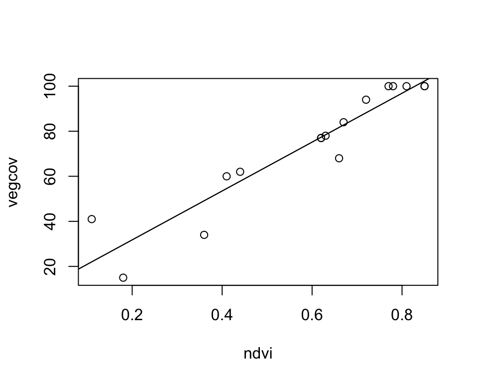
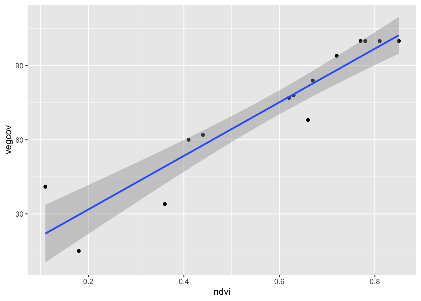
The ggplot version also shows the confidence band around the regression line:
ggplot(train_ds, aes(x = ndvi, y = vegcov)) +
  geom_point() +
  geom_smooth(method = "lm")