library(caret) # cross-validation
library(terra) # reading canopy height model
library(sf) # reading field plots geopackage16 Biomass mapping
Packages
Multiple regression
We will illustrate the multiple regression on data from 50 U.S. states. The variables are population estimate as of July 1, 1975, per capita income (1974), illiteracy (1970, percent of population), life expectancy in years (1969-71), murder and non-negligent manslaughter rate per 100,000 population (1976), percent high-school graduates (1970), mean number of days with min temperature 32 degrees (1931- 1960) in capital or large city, and land area in square miles. The data was collected from US Bureau of the Census. We will take life expectancy as the response and the remaining variables as predictors. (from Faraway, 2002).
data("state")

# a fix is necessary to remove spaces in some of the variable names
statedata <- data.frame(state.x77, row.names=state.abb, check.names=T)
head(statedata)
Population Income Illiteracy Life.Exp Murder HS.Grad Frost Area
AL 3615 3624 2.1 69.05 15.1 41.3 20 50708
AK 365 6315 1.5 69.31 11.3 66.7 152 566432
AZ 2212 4530 1.8 70.55 7.8 58.1 15 113417
AR 2110 3378 1.9 70.66 10.1 39.9 65 51945
CA 21198 5114 1.1 71.71 10.3 62.6 20 156361
CO 2541 4884 0.7 72.06 6.8 63.9 166 103766You can evaluate the correlation between all variables by applying the cor() function to a data frame. With the methods argument, you can chose between “pearson” (default), “kendall”, and “spearman” correlation coefficient.
cor(statedata) Population Income Illiteracy Life.Exp Murder HS.Grad Frost Area
Population 1.000 0.208 0.108 -0.068 0.344 -0.098 -0.332 0.023
Income 0.208 1.000 -0.437 0.340 -0.230 0.620 0.226 0.363
Illiteracy 0.108 -0.437 1.000 -0.588 0.703 -0.657 -0.672 0.077
Life.Exp -0.068 0.340 -0.588 1.000 -0.781 0.582 0.262 -0.107
Murder 0.344 -0.230 0.703 -0.781 1.000 -0.488 -0.539 0.228
HS.Grad -0.098 0.620 -0.657 0.582 -0.488 1.000 0.367 0.334
Frost -0.332 0.226 -0.672 0.262 -0.539 0.367 1.000 0.059
Area 0.023 0.363 0.077 -0.107 0.228 0.334 0.059 1.000Specification of a multiple regression analysis is done by setting up a model formula with + between the explanatory variables. The + means, we are constructing a model that is additive in its predictor variables.
g_step <- lm(Life.Exp ~ Population + Murder, data = statedata)
summary(g_step)
Call:
lm(formula = Life.Exp ~ Population + Murder, data = statedata)

Residuals:
     Min       1Q   Median       3Q      Max
-1.73194 -0.40907 -0.06544  0.48865  2.58417

Coefficients:
              Estimate Std. Error t value Pr(>|t|)
(Intercept)  7.289e+01  2.585e-01 282.012  < 2e-16 ***
Population   6.828e-05  2.742e-05   2.490   0.0164 *
Murder      -3.123e-01  3.317e-02  -9.417 2.15e-12 ***
---
Signif. codes:  0 '***' 0.001 '**' 0.01 '*' 0.05 '.' 0.1 ' ' 1

Residual standard error: 0.8048 on 47 degrees of freedom
Multiple R-squared:  0.6552,    Adjusted R-squared:  0.6405
F-statistic: 44.66 on 2 and 47 DF,  p-value: 1.357e-11
Cross validation
We will use the caret package to perform cross-validation (Kuhn, 2022). The package contains tools for data splitting, pre-processing, feature selection, model tuning using resampling, and variable importance estimation. Here, we use caret’s train() function, which combines model fitting and cross-validation. The function takes a formula and method as input, e.g., lm for linear regression and rf for random forest. How the model is fitted and cross-validated is specified via the trControl argument. The argument takes a list that can be generated with the trainControl() function. Here, we define leave-one-out cross-validation (LOOCV) for training and evaluating the model.
train.control <-  caret::trainControl(method="LOOCV")

lifecv <- caret::train(Life.Exp ~ Population + Murder, data = statedata,
                      method = "lm", trControl = train.control)
lifecv
Linear Regression
50 samples
2 predictor
No pre-processing
Resampling: Leave-One-Out Cross-Validation
Summary of sample sizes: 49, 49, 49, 49, 49, 49, ...
Resampling results:
RMSE Rsquared MAE
0.825422 0.6149637 0.6495435
Tuning parameter 'intercept' was held constant at a value of TRUE
Note
\(R^2\) is calculated by caret by computing the correlation between the observed and predicted values (i.e. R) and squaring the value. When the model is poor, this can lead to differences between this estimator and the more widely known \(R^2\) derived form linear regression models.
Let’s calculate the \(R^2\) based on the sum-of-squares and compare it to the \(R^2\) from caret’s LOOCV. You see the values are different.
lmd <-  lm(Life.Exp ~ Population + Murder, data = statedata)
summary(lmd)[["r.squared"]]
[1] 0.6552033Prediction accuracy
The train() function returns a list (here lifecv) that contains a bunch of results. The summary() function printed the LOOCV prediction errors. We can also access the root-mean-squared error (RMSE) and mean-squared error (MAE) directly from lifecv:
lifecv$results intercept RMSE Rsquared MAE
1 TRUE 0.825422 0.6149637 0.6495435A good way to visually evaluate the prediction accuracy of our model is to plot the predicted vs observed values. In our case, the predicted values were obtained via LOOCV. The list lifecv contains a data.frame pred that we can access as follows:
head(lifecv$pred) pred obs rowIndex intercept
AL 68.33306 69.05 1 TRUE
AK 69.39530 69.31 2 TRUE
AZ 70.60942 70.55 3 TRUE
AR 69.84721 70.66 4 TRUE
CA 70.84711 71.71 5 TRUE
CO 70.91638 72.06 6 TRUEplot(lifecv$pred$pred, lifecv$pred$obs, xlab="Predicted", ylab="Observed")
abline(0,1)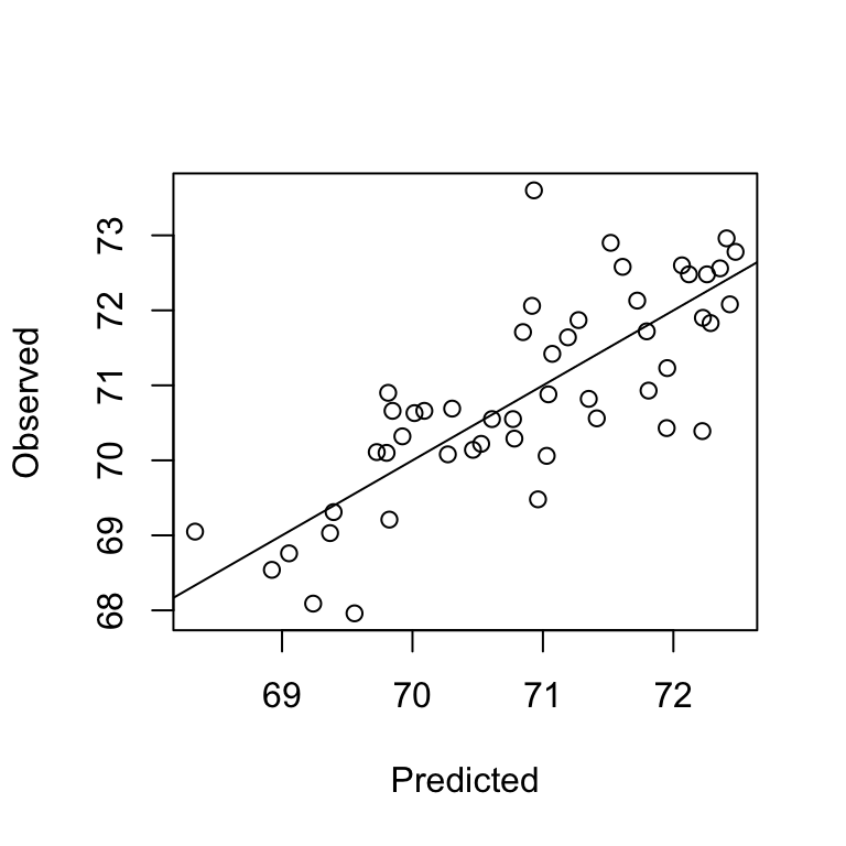
We can also estimate the prediction error (RMSE) manually, and calculate the relative RMSE.
rmse <- function(x,y) sqrt(mean((x-y)^2, na.rm=T))

rmse(lifecv$pred$obs, lifecv$pred$pred)
[1] 0.825422# relative RMSE%
100 * rmse(lifecv$pred$obs, lifecv$pred$pred)/mean(lifecv$pred$obs)[1] 1.164557K-fold cross validation
To conduct a k-fold cross-validation instead of a LOOCV, we simply change the trainControl as follows:
train.control <-  caret::trainControl(method="cv", number = 5)

cv5 <- caret::train(Life.Exp ~ Population + Murder, data = statedata,
                    method = "lm", trControl = train.control)
cv5
Linear Regression
50 samples
2 predictor
No pre-processing
Resampling: Cross-Validated (5 fold)
Summary of sample sizes: 40, 41, 39, 41, 39
Resampling results:
RMSE Rsquared MAE
0.8062673 0.6513883 0.6538312
Tuning parameter 'intercept' was held constant at a value of TRUELidar data
For the study area, we have a canopy height model with a 1m x 1m spatial resolution.
lidar_chm <- rast("data/lidar/yuba_lidar_chm.tif")
lidar_chm
class : SpatRaster
size : 11001, 10001, 1 (nrow, ncol, nlyr)
resolution : 1, 1 (x, y)
extent : 683000, 693001, 4385999, 4397000 (xmin, xmax, ymin, ymax)
coord. ref. : WGS 84 / UTM zone 10N (EPSG:32610)
source : yuba_lidar_chm.tif
name : Layer_1
min value : 0.00000
max value : 79.97305 To fill the background value, which is zero, we use the NAflag function:
NAflag(lidar_chm) <- 0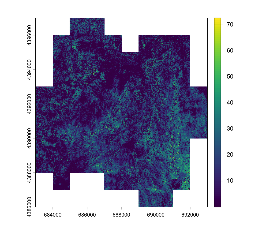
Field biomass
The field data is stored in a geopackage, which we can load into R using the read_sf function from the sf package. Unlike a shapefile, a geopackage can contain multiple layers. The yuba.gpkg contains a polygon layer of the study area boundary (layer=boundary), a polygon layer of the circular field plot boundaries (layer=field_plots), and a point layer of the field plot center locations (layer=field_plot_centers). To read the correct layer, we first need to identify the names and then supply read_sf with the layer name.
st_layers("data/lidar/yuba.gpkg")Driver: GPKG
Available layers:
layer_name geometry_type features fields crs_name
1 boundary Multi Polygon 1 4 WGS 84 / UTM zone 10N
2 field_plots Multi Polygon 39 3 WGS 84 / UTM zone 10N
3 field_plot_centers Point 39 3 WGS 84 / UTM zone 10Nfieldplots <- read_sf("data/lidar/yuba.gpkg", "field_plots")
fieldplotsSimple feature collection with 39 features and 3 fields
Geometry type: MULTIPOLYGON
Dimension: XY
Bounding box: xmin: 684133.3 ymin: 4387457 xmax: 691676.7 ymax: 4394925
Projected CRS: WGS 84 / UTM zone 10N
# A tibble: 39 × 4
grid_ptn grid_id lagb_t_ha geom
<chr> <int> <dbl> <MULTIPOLYGON [m]>
1 B7 7 241. (((684151.2 4388713, 684154.4 4388713, 684157.4 4388712, 684160.2 438…
2 B6 6 281. (((684158.6 4390108, 684161.7 4390108, 684164.7 4390107, 684167.6 439…
3 B4 4 201. (((684159.7 4392466, 684162.8 4392466, 684165.8 4392465, 684168.7 439…
4 B5 5 553. (((684160 4391219, 684163.2 4391219, 684166.2 4391218, 684169 4391217…
5 C7 13 153. (((685118.7 4388716, 685121.8 4388715, 685124.8 4388714, 685127.7 438…
6 C2 8 157. (((685396.4 4394854, 685399.5 4394853, 685402.5 4394853, 685405.3 439…
7 C6 12 517. (((685405.6 4389960, 685408.7 4389960, 685411.8 4389959, 685414.6 438…
8 C5 11 191. (((685406.6 4391214, 685409.7 4391214, 685412.8 4391213, 685415.6 439…
9 C4 10 917. (((685404.2 4392459, 685407.3 4392459, 685410.4 4392458, 685413.2 439…
10 C3 9 211. (((685409.8 4393718, 685413 4393718, 685416 4393717, 685418.8 4393716…
# ℹ 29 more rowsWe can add the plot location atop the image:
plot(lidar_chm)
plot(st_geometry(fieldplots), add=T)
Extract lidar metrics
Using the extract function in the terra package we can calculate statistical summaries of all pixels within each plot polygon. Previously, we’ve used the extract function to extract single pixel values associated with point locations. When supplying extract() with a polygon layer, we should also specify the fun argument, i.e., the aggregation function that should be applied to all values in each polygon. Here, we calculate the mean canopy height for each plot polygon.
plots_htmean <- extract(x = lidar_chm, y = fieldplots, fun = mean, ID=F)
head(plots_htmean)
Layer_1
1 9.643645
2 9.600241
3 7.756380
4 21.687645
5 7.451048
6 9.878860We can define any type of function. Let’s extract the 50th percentile of CHM values for each field plot polygon.
plots_pc50 <- extract(x = lidar_chm, y = fieldplots, ID=F,
                      fun = function(x, na.rm=T) quantile(x, 0.5, na.rm=T))
head(plots_pc50)
Layer_1
1 7.5137088
2 7.1726367
3 0.8170152
4 22.7622108
5 7.2014172
6 9.9030981To train a model, we need to combine the lidar metrics (predictors) and the field biomass (response) in a single data.frame.
dfplots <- cbind(fieldplots[, c("grid_id", "lagb_t_ha")],
                 htmean = plots_htmean[,1], htpc50 = plots_pc50[,1])

head(dfplots)
Simple feature collection with 6 features and 4 fields
Geometry type: MULTIPOLYGON
Dimension: XY
Bounding box: xmin: 684133.3 ymin: 4388677 xmax: 685414.3 ymax: 4394854
Projected CRS: WGS 84 / UTM zone 10N
grid_id lagb_t_ha htmean htpc50 geom
1 7 240.6803 9.643645 7.5137088 MULTIPOLYGON (((684151.2 43...
2 6 280.7319 9.600241 7.1726367 MULTIPOLYGON (((684158.6 43...
3 4 201.2614 7.756380 0.8170152 MULTIPOLYGON (((684159.7 43...
4 5 552.8304 21.687645 22.7622108 MULTIPOLYGON (((684160 4391...
5 13 153.4288 7.451048 7.2014172 MULTIPOLYGON (((685118.7 43...
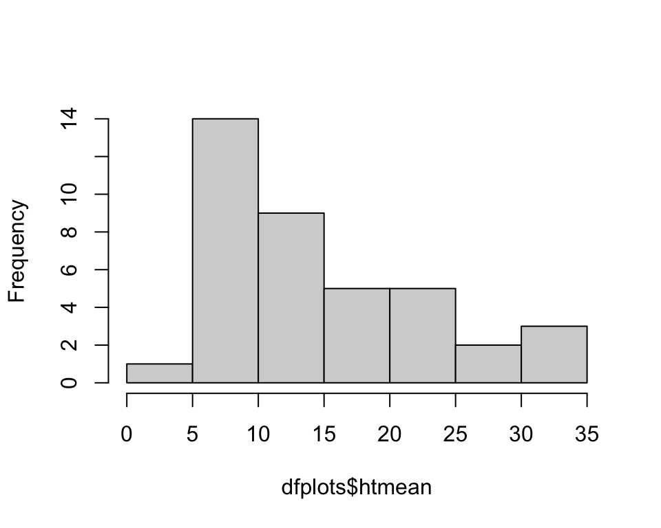
6 8 157.1963 9.878860 9.9030981 MULTIPOLYGON (((685396.4 43...Histogram of mean CHM height:
hist(dfplots$htmean, main='')