library(terra)6 Raster data
Raster consist of cells (pixels) that are arranged as rows and columns in a regular grid. Examples of raster data are digital elevation models (DEM), gridded climate or meteorological variables, satellite images, discrete maps such as land cover maps, and continuous maps of vegetation cover, biophysical variables, and soil variables. Common raster file formats are the GeoTiff (.tif), IMAGINE (.img), and NetCDF (.nc). There are many more formats, but most of them can be read and written in R.
terra
The terra package is the main package for creating, reading, manipulating, and writing raster data (Hijmans, 2024). The terra package supersedes the older raster package developed by the same team of authors. Because raster has been around for a longer time, dependencies with some packages may still exist. But development of raster will eventually be stopped at some point. You’ll find an online documentation of the package here. I also recommend you scroll through the package description to get a first overview of the functationality of the package.
?`terra-package`The terra package defines a number of spatial classes. The most important ones are:
SpatRasterto store raster dataSpatVectorto store spatial vector data, i.e., points, lines, polygons.SpatExtentto store information on spatial extent
HyMap data
In this chapter, we use imaging spectrometer data acquired by the HyMap sensor during the HyEurope 2009 campaign of the German Aerospace Center (DLR) on 20 August 2009. The aircraft flew over Berlin at an altitude of approximately 4,750 m, resulting in a spatial resolution of 9 m × 9 m after ortho-rectification. Pre-processing to surface reflectance included system and radiometric correction. To reduce noise in subsequent analyses, the original 128 spectral bands were reduced to 111.
HyMap (Hyperspectral Mapper) is an airborne imaging spectrometer designed for high-resolution hyperspectral remote sensing. It comprises four spectrometers covering the 0.45–2.45 µm range, excluding the two major atmospheric water-absorption regions.
Read and create
The rast function creates a SpatRaster object. A SpatRaster can be generated from scratch, from a file, or from an existing R object.
Usually, we create a SpatRaster object from a filename (or a vector of file names if the bands are stored in separate filenames). The resulting object (here hymap) represents a connection to the physical file on disc, but does not store the file in memory. This is helpful when opening large raster files. Type the object into the console to print important metadata of the raster including dimensions, coordinate reference system, extent, layer names.
hymap <- rast("data/frac/HyMap02_Berlin_2009_subset.bsq")
hymap
class : SpatRaster
size : 730, 730, 111 (nrow, ncol, nlyr)
resolution : 9, 9 (x, y)
extent : 380982.4, 387552.4, 5810457, 5817027 (xmin, xmax, ymin, ymax)
coord. ref. : UTM_Zone_33N
source : HyMap02_Berlin_2009_subset.bsq
names : 0.455400, 0.469400, 0.484300, 0.499100, 0.513800, 0.528800, ... Notice the wavelength are stored in the layer names:
names(hymap) [1] "0.455400" "0.469400" "0.484300" "0.499100" "0.513800" "0.528800"
[7] "0.543600" "0.558400" "0.573100" "0.588100" "0.602900" "0.617600"
[13] "0.632000" "0.646500" "0.660900" "0.675500" "0.690000" "0.704500"
[19] "0.718900" "0.733200" "0.747600" "0.761800" "0.775900" "0.790100"
[25] "0.804600" "0.818800" "0.832900" "0.847100" "0.861100" "0.874700"
[31] "0.887800" "0.893000" "0.908500" "0.923900" "0.939400" "0.955200"
[37] "0.970400" "0.985800" "1.001400" "1.016600" "1.031800" "1.046900"
[43] "1.062000" "1.076600" "1.091300" "1.106200" "1.120800" "1.135300"
[49] "1.149700" "1.164100" "1.178600" "1.192800" "1.206900" "1.221000"
[55] "1.235100" "1.249200" "1.263100" "1.277000" "1.290700" "1.304300"
[61] "1.318300" "1.330100" "1.505000" "1.518800" "1.532600" "1.546300"
[67] "1.559800" "1.573200" "1.586400" "1.599500" "1.612700" "1.625900"
[73] "1.638900" "1.651700" "1.664400" "1.677100" "1.689600" "1.702100"
[79] "1.714600" "1.726900" "1.739300" "1.751500" "1.763600" "1.775600"
[85] "1.787600" "1.798100" "2.027500" "2.046700" "2.065500" "2.084100"
[91] "2.102500" "2.120900" "2.139000" "2.157000" "2.174700" "2.191700"
[97] "2.210300" "2.228100" "2.245600" "2.263400" "2.280400" "2.297400"
[103] "2.314400" "2.331400" "2.348300" "2.365000" "2.381500" "2.397700"
[109] "2.414100" "2.430300" "2.446500"Missing values
We may also need to take care of NA values. The information which numeric values represent NA may get lost when importing the raster image, or this information was not present in the metadata. NA (or background) values are often very high/low values or zero (but not always).
# The output tells us that no numeric value has been declared as 'NA'
NAflag(hymap)
[1] NaN# let R know that Zeros are nodata values: NA
NAflag(hymap) <- 0Layers
We may want to access individual layers (bands) of an image in order to manipulate them, for example for transformations or the calculation of spectral indices. We can access individual layers using the $ operator followed by the layer name, similar to accessing columns in a data.frame. Note that in the example below, we need to wrap the layer name in backticks because it contains an unsupported character (.).
band1 <- hymap$`0.455400`Alternatively, using numeric indexing:
hymap_red <- hymap[[15]] # red bandOr using subset():
hymap_nir <- subset(hymap, 30) # NIR bandPlot
Applying plot() to a multi-layer raster creates a panel plot where each layer is visualized in a separate subplot. Note, the argument nc specifies the number of columns of the panel plot.
plot(hymap, nc=4, maxnl=4)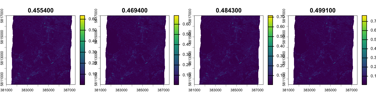
Alternatively, you can specify the numeric id’s of the layers you want to plot. The code below plots only layer 1.
plot(hymap, 1)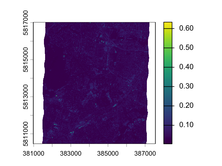
Using the plotRGB function we can create an RGB representation of three image bands:
plotRGB(hymap, r = 75, g= 28, b = 15, stretch='hist')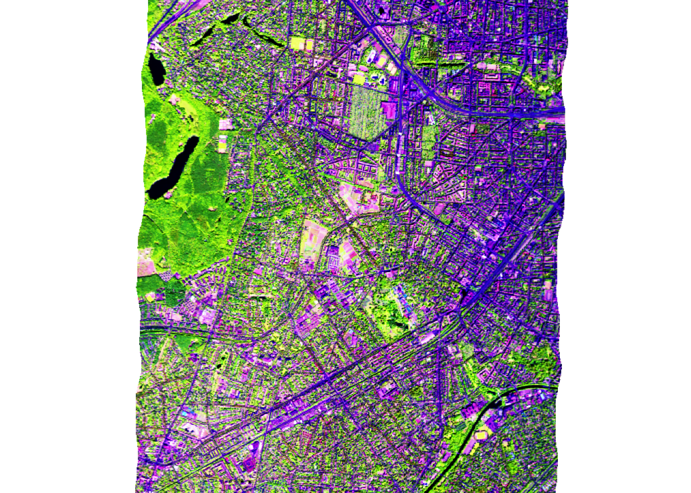
We can plot two bands against each other with plot(). Note that the function only uses a random sample of the raster values to create the plot. You can adjust the number of pixels plotted with the maxcell argument.
plot(hymap_red, hymap_nir)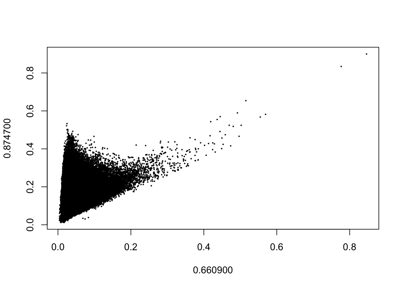
Manipulate
We can manipulate the pixel values of a layer by applying basic functions and operations.
hymap_nir_scaled <- 100 * hymap_nir^2
plot(hymap_nir_scaled)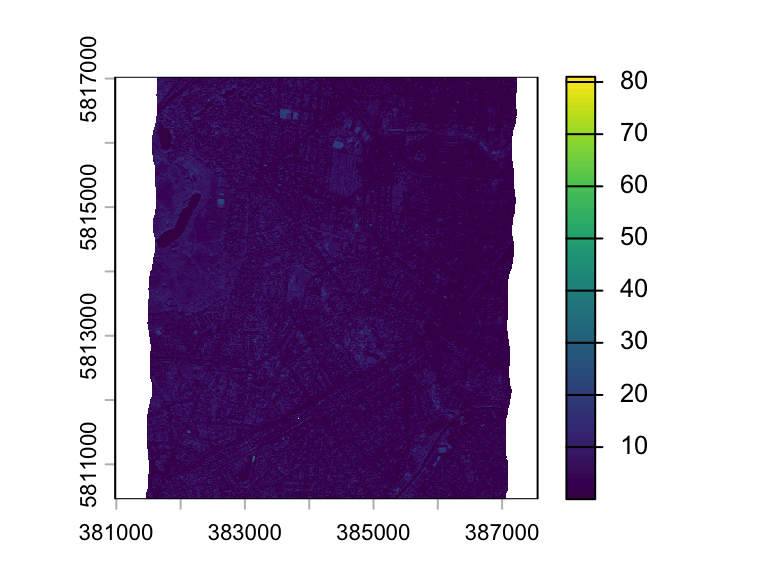
We can perform arithmetic operations between layers:
ndvi <- (hymap_nir - hymap_red) / (hymap_red + hymap_nir)
plot(ndvi)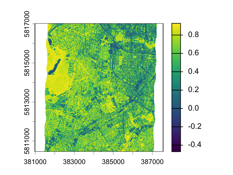
We can apply a logical expression to create a binary mask:
mask <- ndvi > 0.2
plot(mask)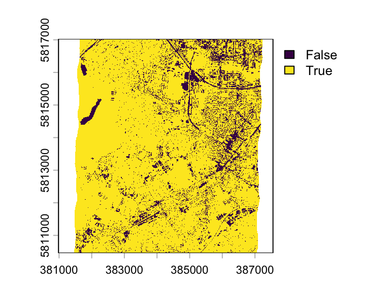
Stack
We can stack multiple layers (SpatRaster) together using the concatenate function c().
img <- c(hymap_red, hymap_nir)

# assign meaningful names to the layers
names(img) <- c("Red", "Near-IR")

plot(img)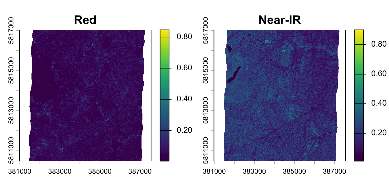
Statistics
Summary functions (min, max, mean, prod, sum, median, cv, any, all) yield a single value for every pixel (or two values when using range). So, they always return a SpatRaster object with a single layer (or two layers in case of range). The following code calculates for every pixel in SpatRaster img, the mean value across the two layers.
img_mean <- mean(img)
plot(img_mean)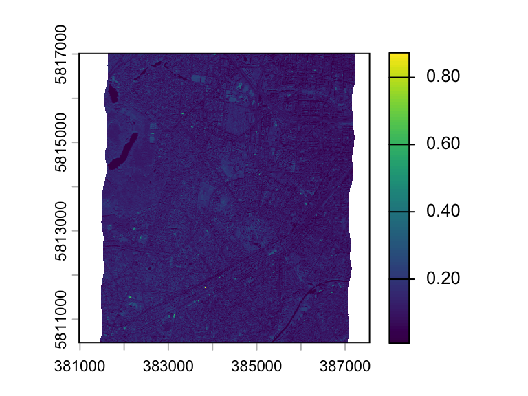
If you want a single value summarizing all pixel values, e.g. mean pixel value for each layer, use global.
global(img, fun="mean", na.rm = TRUE) mean
Red 0.05246533
Near-IR 0.18924152Masking
You can use the square brackets to access and replace values in a raster. The example below shows how to truncate a value range: all values less than 0 are replaced with the 0.
ndvi[ndvi < 0] <- 0
plot(ndvi)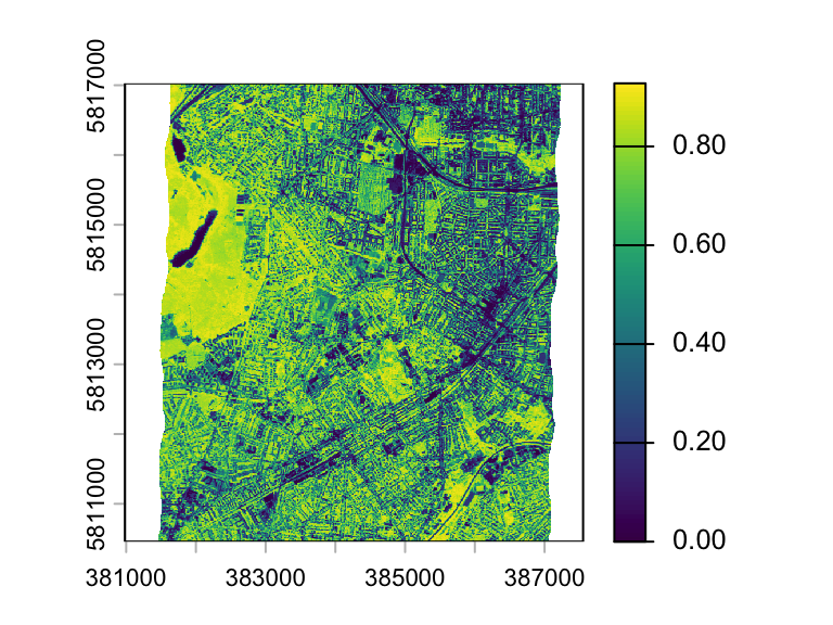
The expression ndvi < 0 creates a binary mask that identifies the pixels to be replaced. Here, we make the creation of the mask more explicit:
mask <- ndvi < 0
ndvi[mask] <- 0
Apply
The function app provides a more generic interface to do a computation for a single SpatRaster. The function takes a SpatRaster and the function you want to apply. The function below replaces all values less than and equal to 0.1 with NA. Note, this is just a simple example. The idea here is to facilitate the application of more complex functions from you or other packages.
myFunction <- function(x){ x[x <= 0.1] <- NA; return(x)}
img2 <- app(img, fun= myFunction)
plot(img2, range=c(0,1))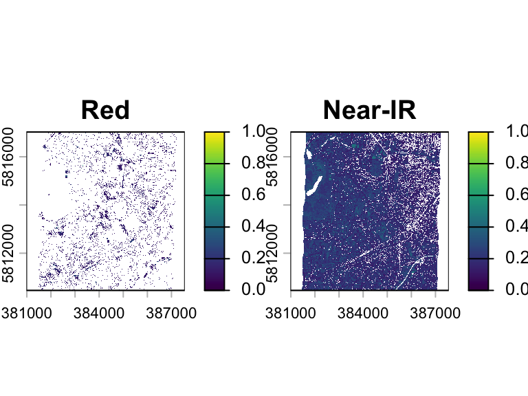
Recode
We can recode raster values using the classify function terra. The term classify can be a bit confusing, as it essentially creates a classification by binning values. This is useful when you want to: 1) bin continuous value ranges into discrete classes, or 2) recode discrete values, such as land cover codes, into new values.
To translate old value ranges or values into new values, we need to create a matrix. The three columns represent the from value range (1), the to value range (2), and the new class value (3). For example, values from -0.1 to 1.2 will be classified to 1.
k <- matrix(c(-1.0, 0.0, 1,
               0.0, 0.3, 2,
               0.3, 1.0, 3),
            ncol = 3, byrow = TRUE)
k
[,1] [,2] [,3]
[1,] -1.0 0.0 1
[2,] 0.0 0.3 2
[3,] 0.3 1.0 3Using this matrix as a look-up table, we can classify the raster object:
rast_class <- terra::classify(x= ndvi, rcl = k)
plot(rast_class, type='classes')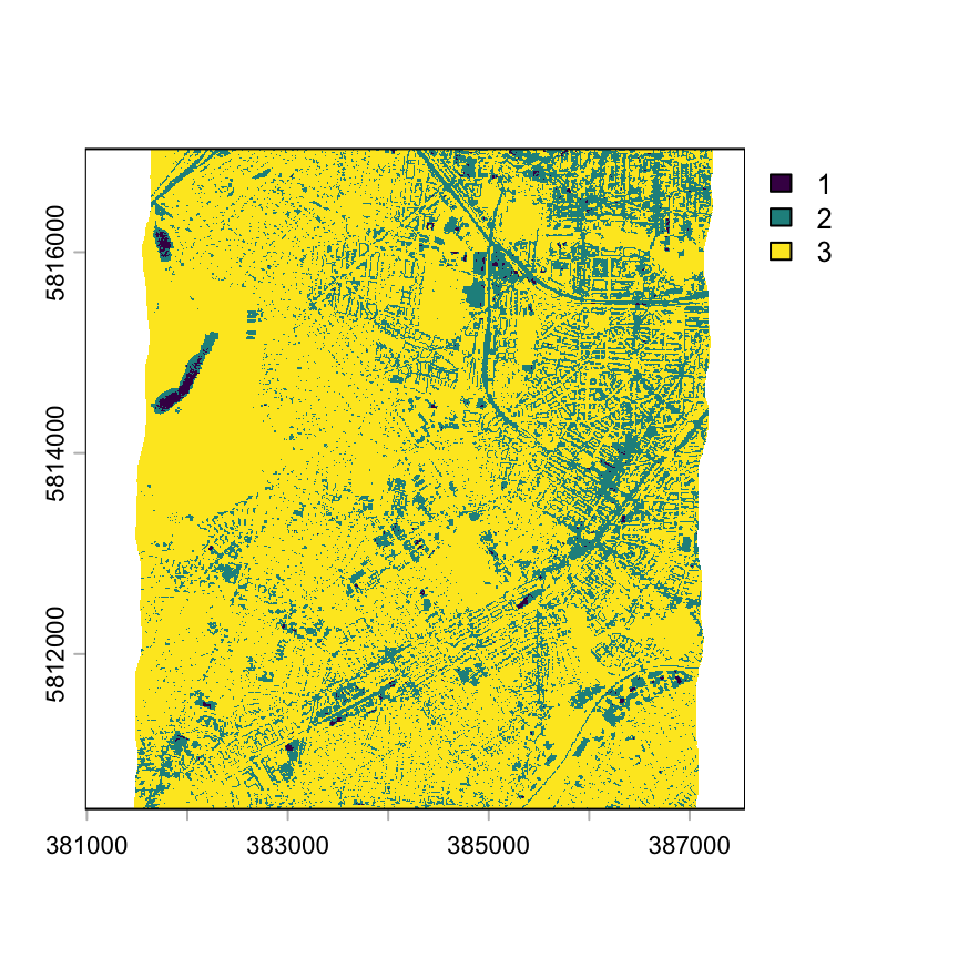
Write
Use writeRaster to save a SpatRaster to a file. To overwrite an existing file, use overwrite = TRUE. The file type is usually inferred from the filename extension, but if needed, you can specify it explicitly with, for example, format = "GTiff". Type gdal(drivers=TRUE) in your console to see what file types are available in your installation.
writeRaster(hymap, "hymap_output.tif", overwrite=TRUE)You can define the ouput data type with the argument datatype. Choosing an appropriate data type can help minimize disk space usage. For instance, a land cover map usually has values no larger than 255, so using an 8-bit integer (INT1U) requires only half the storage of a 16-bit integer (INT2) and a quarter of that of a 32-bit float (FLT4S).
| Data type | Description | Value range |
|---|---|---|
| INT1S | 8-bit signed integer | -128 to 127 |
| INT1U | 8-bit unsigned integer | 0 to 255 |
| INT2S | 16-bit signed integer | -32,768 to 32,767 |
| INT2U | 16-bit unsigned integer | 0 to 65,535 |
| INT4S | 32-bit signed integer | -2,147,483,648 to 2,147,483,647 |
| INT4U | 32-bit unsigned integer | 0 to 4,294,967,295 |
| FLT4S | 32-bit floating point | ±3.4 × 10³⁸ (approx.) |
| FLT8S | 64-bit floating point | ±1.8 × 10³⁰⁸ (approx.) |
Sampling
Raster can have millions of pixels, which can make computations very slow. So, sometimes it is useful to do calculations only on a sample of the raster pixels, e.g., for estimating raster statistics or for building a statistical model. The spatSample function can be used to extract a random sample and stratified sample. If you want to retrieve the same random sample every time you re-run spatSample, set the random seed to the same number. This is helpful when debugging your code, and you want to exclude random variations during your testing.
set.seed(42)
hymap_sample <- spatSample(hymap, size=1000, method="random")
head(hymap_sample)
0.455400 0.469400 0.484300 0.499100 0.513800 0.528800 0.543600 0.558400 0.573100 0.588100 0.602900 0.617600 0.632000 0.646500 0.660900 0.675500 0.690000 0.704500 0.718900 0.733200 0.747600 0.761800 0.775900 0.790100 0.804600 0.818800 0.832900 0.847100 0.861100 0.874700 0.887800 0.893000 0.908500 0.923900 0.939400 0.955200 0.970400 0.985800 1.001400 1.016600 1.031800 1.046900 1.062000 1.076600 1.091300 1.106200 1.120800 1.135300 1.149700 1.164100 1.178600 1.192800 1.206900 1.221000 1.235100 1.249200 1.263100 1.277000 1.290700 1.304300 1.318300 1.330100 1.505000 1.518800 1.532600 1.546300 1.559800 1.573200 1.586400 1.599500 1.612700 1.625900 1.638900 1.651700 1.664400 1.677100 1.689600 1.702100 1.714600 1.726900 1.739300 1.751500 1.763600 1.775600 1.787600 1.798100 2.027500 2.046700 2.065500 2.084100 2.102500 2.120900 2.139000 2.157000 2.174700 2.191700 2.210300 2.228100 2.245600 2.263400 2.280400 2.297400 2.314400 2.331400 2.348300 2.365000 2.381500 2.397700 2.414100 2.430300 2.446500
1 NA NA NA NA NA NA NA NA NA NA NA NA NA NA NA NA NA NA NA NA NA NA NA NA NA NA NA NA NA NA NA NA NA NA NA NA NA NA NA NA NA NA NA NA NA NA NA NA NA NA NA NA NA NA NA NA NA NA NA NA NA NA NA NA NA NA NA NA NA NA NA NA NA NA NA NA NA NA NA NA NA NA NA NA NA NA NA NA NA NA NA NA NA NA NA NA NA NA NA NA NA NA NA NA NA NA NA NA NA NA NA
2 0.0153 0.0163 0.0165 0.0160 0.0191 0.0222 0.0248 0.0252 0.0231 0.0214 0.0205 0.0189 0.0177 0.0169 0.0155 0.0171 0.0422 0.0695 0.0966 0.1233 0.1493 0.1615 0.1717 0.1756 0.1790 0.1823 0.1855 0.1886 0.1902 0.1915 0.1937 0.1938 0.1938 0.1935 0.1918 0.1898 0.1897 0.1926 0.1960 0.2013 0.2085 0.2116 0.2135 0.2144 0.2111 0.2063 0.2001 0.1899 0.1769 0.1678 0.1671 0.1676 0.1709 0.1749 0.1795 0.1832 0.1864 0.1866 0.1815 0.1726 0.1606 0.1520 0.0488 0.0552 0.0610 0.0663 0.0709 0.0758 0.0790 0.0825 0.0858 0.0882 0.0903 0.0914 0.0917 0.0901 0.0888 0.0855 0.0825 0.0802 0.0785 0.0754 0.0726 0.0684 0.0617 0.0585 0.0248 0.0275 0.0295 0.0317 0.0334 0.0355 0.0369 0.0379 0.0393 0.0409 0.0418 0.0413 0.0405 0.0379 0.0345 0.0310 0.0306 0.0281 0.0270 0.0246 0.0234 0.0193 0.0184 0.0163 0.0141
3 NA NA NA NA NA NA NA NA NA NA NA NA NA NA NA NA NA NA NA NA NA NA NA NA NA NA NA NA NA NA NA NA NA NA NA NA NA NA NA NA NA NA NA NA NA NA NA NA NA NA NA NA NA NA NA NA NA NA NA NA NA NA NA NA NA NA NA NA NA NA NA NA NA NA NA NA NA NA NA NA NA NA NA NA NA NA NA NA NA NA NA NA NA NA NA NA NA NA NA NA NA NA NA NA NA NA NA NA NA NA NA
4 0.0702 0.0724 0.0742 0.0764 0.0777 0.0800 0.0838 0.0920 0.1027 0.1154 0.1264 0.1320 0.1359 0.1390 0.1425 0.1458 0.1504 0.1551 0.1598 0.1644 0.1688 0.1704 0.1714 0.1706 0.1695 0.1684 0.1673 0.1661 0.1643 0.1629 0.1659 0.1666 0.1712 0.1756 0.1799 0.1843 0.1884 0.1926 0.1971 0.2030 0.2071 0.2107 0.2142 0.2162 0.2185 0.2210 0.2233 0.2255 0.2277 0.2298 0.2331 0.2364 0.2392 0.2425 0.2444 0.2466 0.2491 0.2523 0.2485 0.2445 0.2426 0.2408 0.2418 0.2503 0.2556 0.2589 0.2616 0.2635 0.2637 0.2643 0.2639 0.2644 0.2652 0.2641 0.2651 0.2652 0.2650 0.2640 0.2624 0.2623 0.2608 0.2582 0.2583 0.2562 0.2559 0.2552 0.2658 0.2880 0.2807 0.2837 0.2873 0.2874 0.2893 0.2870 0.2846 0.2817 0.2810 0.2846 0.2853 0.2872 0.2857 0.2845 0.2834 0.2778 0.2687 0.2679 0.2624 0.2597 0.2551 0.2469 0.2525
5 0.0707 0.0739 0.0740 0.0764 0.0781 0.0786 0.0802 0.0825 0.0842 0.0860 0.0869 0.0876 0.0889 0.0896 0.0898 0.0913 0.0939 0.0966 0.0992 0.1019 0.1044 0.1053 0.1060 0.1067 0.1074 0.1081 0.1088 0.1093 0.1088 0.1107 0.1115 0.1116 0.1125 0.1133 0.1141 0.1149 0.1157 0.1165 0.1174 0.1190 0.1208 0.1220 0.1225 0.1224 0.1226 0.1229 0.1231 0.1232 0.1232 0.1233 0.1240 0.1249 0.1267 0.1281 0.1300 0.1324 0.1349 0.1347 0.1339 0.1336 0.1302 0.1289 0.1239 0.1272 0.1304 0.1323 0.1333 0.1345 0.1348 0.1359 0.1362 0.1367 0.1361 0.1367 0.1360 0.1357 0.1352 0.1344 0.1338 0.1320 0.1314 0.1299 0.1280 0.1249 0.1241 0.1236 0.1264 0.1291 0.1304 0.1300 0.1300 0.1299 0.1284 0.1269 0.1252 0.1236 0.1234 0.1226 0.1203 0.1196 0.1165 0.1112 0.1087 0.1059 0.1016 0.1007 0.0997 0.0981 0.0960 0.0970 0.0904
6 0.0159 0.0156 0.0157 0.0165 0.0190 0.0241 0.0276 0.0281 0.0249 0.0221 0.0211 0.0193 0.0188 0.0173 0.0161 0.0193 0.0587 0.1015 0.1439 0.1857 0.2265 0.2478 0.2660 0.2718 0.2763 0.2808 0.2852 0.2895 0.2926 0.2969 0.2999 0.3001 0.3004 0.3004 0.2985 0.2963 0.2960 0.3001 0.3051 0.3138 0.3209 0.3278 0.3313 0.3313 0.3270 0.3211 0.3133 0.2997 0.2823 0.2700 0.2719 0.2754 0.2798 0.2867 0.2958 0.3048 0.3114 0.3110 0.3057 0.2981 0.2815 0.2667 0.0842 0.0946 0.1054 0.1149 0.1233 0.1310 0.1378 0.1446 0.1503 0.1555 0.1589 0.1603 0.1594 0.1582 0.1540 0.1484 0.1422 0.1361 0.1333 0.1286 0.1236 0.1186 0.1072 0.1016 0.0375 0.0402 0.0443 0.0474 0.0507 0.0534 0.0554 0.0572 0.0595 0.0622 0.0653 0.0651 0.0618 0.0565 0.0506 0.0457 0.0428 0.0405 0.0367 0.0344 0.0316 0.0288 0.0262 0.0234 0.0193Let’s plot the red and NIR band pixels from the sample (data.frame) against each other:
plot(hymap_sample[,15], hymap_sample[,30], xlab="Red", ylab="NIR")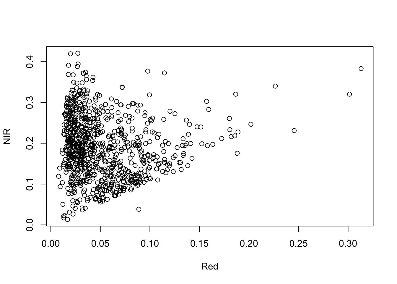
Note
The function spatSample returns by default a data.frame, but it can also return a SpatVector object (as.points=T) or raster object (as.raster=T).
Plot pixel spectra
We want to plot the spectra for three different surfaces: water, conifer forest, road, grass, clay-tile roof. To plot the spectra, we first need to obtain the wavelength information from the band names and convert them into numeric values.
wavelength <- names(hymap)
wavelength <- as.numeric(wavelength)
wavelength
[1] 0.4554 0.4694 0.4843 0.4991 0.5138 0.5288 0.5436 0.5584 0.5731 0.5881
[11] 0.6029 0.6176 0.6320 0.6465 0.6609 0.6755 0.6900 0.7045 0.7189 0.7332
[21] 0.7476 0.7618 0.7759 0.7901 0.8046 0.8188 0.8329 0.8471 0.8611 0.8747
[31] 0.8878 0.8930 0.9085 0.9239 0.9394 0.9552 0.9704 0.9858 1.0014 1.0166
[41] 1.0318 1.0469 1.0620 1.0766 1.0913 1.1062 1.1208 1.1353 1.1497 1.1641
[51] 1.1786 1.1928 1.2069 1.2210 1.2351 1.2492 1.2631 1.2770 1.2907 1.3043
[61] 1.3183 1.3301 1.5050 1.5188 1.5326 1.5463 1.5598 1.5732 1.5864 1.5995
[71] 1.6127 1.6259 1.6389 1.6517 1.6644 1.6771 1.6896 1.7021 1.7146 1.7269
[81] 1.7393 1.7515 1.7636 1.7756 1.7876 1.7981 2.0275 2.0467 2.0655 2.0841
[91] 2.1025 2.1209 2.1390 2.1570 2.1747 2.1917 2.2103 2.2281 2.2456 2.2634
[101] 2.2804 2.2974 2.3144 2.3314 2.3483 2.3650 2.3815 2.3977 2.4141 2.4303
[111] 2.4465We can extract individual pixels using the row and column ID’s. The result is a data.frame with 1 row (observation) and 111 columns (bands). The function t() transposes these data.frames to a matrix of 1 column and 111 rows.
s_water   <- t(hymap[240,120])
s_conifer <- t(hymap[260,150])
s_road    <- t(hymap[170,610])
s_grass   <- t(hymap[645, 565])
s_roof    <- t(hymap[289, 542])
head(s_water)
[,1]
0.455400 0.0101
0.469400 0.0132
0.484300 0.0141
0.499100 0.0146
0.513800 0.0165
0.528800 0.0201Now, let’s plot the spectra using R’s base graphic system:
plot(wavelength, s_water, col='blue', ylim=c(0,0.5), ylab='Reflectance', xlab='Wavelength (nm)')
points(wavelength, s_conifer, col='darkgreen')
points(wavelength, s_road, col='red')
points(wavelength, s_grass, col='green')
points(wavelength, s_roof, col='black')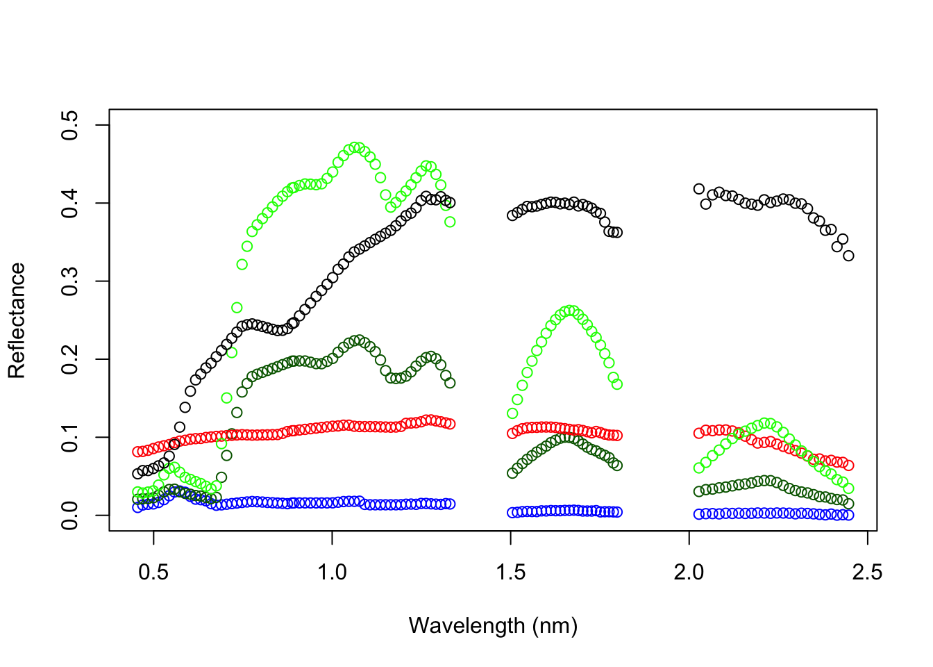
Crop
You can use the bounding box from zoom() or create one with ext() to crop() an image. The cropping may take a while depending on your CPU. Note, that the variable hymap_subset links to a file that was created in R’s temporary directory. It’s not stored in memory.
my_bounding_box <- ext(c(382207.4, 383817.4, 5813147, 5814837))
hymap_subset <- crop(hymap, my_bounding_box)
Predict
The terra package has two functions to make model predictions to (potentially very large) rasters. The function predict takes a multilayer raster and a fitted model as arguments. Fitted models can be of various classes, including lm, glm, gam, RandomForest, and prcomp (PCA). We’ve used predict already to apply linear models to data.frames. The function interpolate is similar but is for models that use coordinates as predictor variables, for example in Kriging and spline interpolation. Type this into the console to see the corresponding help page.
?`predict,SpatRaster-method`Map interaction
The functions zoom() and click() let you interact with your plotted image. Don’t use them in markdown/knitr as these functions wait for interactive input.
The function click() either returns a coordinate, or the value of the image you call it with.
The function zoom() allows you to select a bounding box (upperleft and lowerright corner). The function always returns the spatial extent of the selected bounding box.
my_selected_coordiante <- click()
my_selected_ndvi_value <- click(ndvi)
# press ESC to end interactive mode

# only returns bounding box
my_bounding_box <- zoom()

# returns bounding box and pops-up a zoom window
my_bounding_box <- zoom(ndvi)