library(tidyr)
library(dplyr)
library(ggplot2)4 Data wrangling
Packages
Tidy data
Cleaning and preparing (tidying) data for analysis can make up a substantial proportion of the time spent on a project. It is therefore good practice to follow certain guidelines for structuring your data (Wickham, 2014):
- Each variable forms a column.
- Each observation forms a row.
- Each type of observational unit forms a table.
Real datasets can, and often do, violate the three precepts of tidy data in almost every way imaginable. While occasionally you do get a dataset that you can start analysing immediately, this is the exception, not the rule. This section describes the five most common problems with messy datasets, along with their remedies:
- Column headers are values, not variable names.
- Multiple variables are stored in one column.
- Variables are stored in both rows and columns.
- Multiple types of observational units are stored in the same table.
- A single observational unit is stored in multiple tables.
Basically, data is often recorded in this format (wide-format):
| Plot | Measure1 | Measure2 |
|---|---|---|
| 1 | 13.1 | 12.7 |
| 2 | 9.5 | 10.6 |
| 3 | 11.9 | 7.4 |
But we want to have it in following format (long-format)
| Plot | Measure | Value |
|---|---|---|
| 1 | M1 | 13.1 |
| 2 | M1 | 9.5 |
| 3 | M1 | 11.9 |
| 1 | M2 | 12.7 |
| 2 | M2 | 10.6 |
| 3 | M2 | 7.4 |
In real-world datasets, data is often messy, incomplete, or not structured for analysis. The dplyr and tidyr packages in R provide a set of powerful tools to clean, transform, and reshape data efficiently. dplyr focuses on data manipulation tasks such as filtering, selecting, summarizing, and joining datasets, while tidyr helps reshape data, for example by pivoting tables or separating and combining columns. Together, they make it much easier to turn raw, unorganized data into a format suitable for analysis and visualization. For a quick reference, see the following cheat sheets for tidyr and dplyr.
Reshape
yields <- read.table("data/basic/yields.txt", sep = ";", header = TRUE)
yields[1:5, ]
plotid sand clay loam
1 1 6 17 13
2 2 10 15 16
3 3 8 3 9
4 4 6 11 12
5 5 14 14 15The pivot_longer() function in the tidyr package can be used to convert the previous dataset into a tidy dataset. In the example below, we want to reshape the sand, clay, and loam columns, hence we exclude the plotid column (denoted with a minus sign). See also here, for ways to select columns in the tidyverse.
yields_tidy <- tidyr::pivot_longer(yields, cols= -plotid, names_to = "soiltype", values_to = "yield")

# pivot_longer(yields, cols= starts_with(c("sand", "loam", "clay")), names_to = "soiltype", values_to = "yield")

yields_tidy[c(1:3, 11:13), ]
# A tibble: 6 × 3
plotid soiltype yield
<int> <chr> <int>
1 1 sand 6
2 1 clay 17
3 1 loam 13
4 4 clay 11
5 4 loam 12
6 5 sand 14The dataset is now tidy, i.e. ready for analysis and plotting:
ggplot(yields_tidy, aes(x = soiltype, y = yield)) +
  geom_boxplot()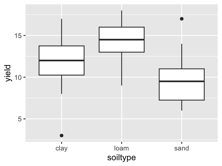
Sometimes we want to back-transform the data into wide format, which can be done using the pivot_wider() function:
yields <- pivot_wider(yields_tidy, id_cols=plotid, names_from=soiltype, values_from=yield)
yields[1:3, ]
# A tibble: 3 × 4
plotid sand clay loam
<int> <int> <int> <int>
1 1 6 17 13
2 2 10 15 16
3 3 8 3 9Sometimes column names include several attributes:
yields2 <- read.table("data/basic/yields2.txt", sep = ";", header = TRUE)
yields2[1:3, ]
plotid sand_fine clay_fine loam_fine sand_coarse clay_coarse loam_coarse
1 1 6 17 13 9 18 15
2 2 10 15 16 10 15 18
3 3 8 3 9 9 3 9After transforming it into long format, the data still is not a tidy data set (‘Multiple variables are stored in one column’):
yields2_tidy <- pivot_longer(yields2, cols= starts_with(c("sand", "loam", "clay")), names_to = "soiltype", values_to = "yield")

yields2_tidy[c(1:3, 11:13), ]
# A tibble: 6 × 3
plotid soiltype yield
<int> <chr> <int>
1 1 sand_fine 6
2 1 sand_coarse 9
3 1 loam_fine 13
4 2 clay_fine 15
5 2 clay_coarse 15
6 3 sand_fine 8separate()
We need to split the soiltype column into two columns soildtype and grain. This can easily be done using the separate() function:
yields2_tidy <- separate(yields2_tidy, col = soiltype, into = c("soiltype", "grain"), sep = "_")
yields2_tidy[c(1:3, 11:13), ]
# A tibble: 6 × 4
plotid soiltype grain yield
<int> <chr> <chr> <int>
1 1 sand fine 6
2 1 sand coarse 9
3 1 loam fine 13
4 2 clay fine 15
5 2 clay coarse 15
6 3 sand fine 8Which can now be nicely plotted using ggplot2:
ggplot(yields2_tidy, aes(x = soiltype, y = yield, fill = grain)) +
  geom_boxplot()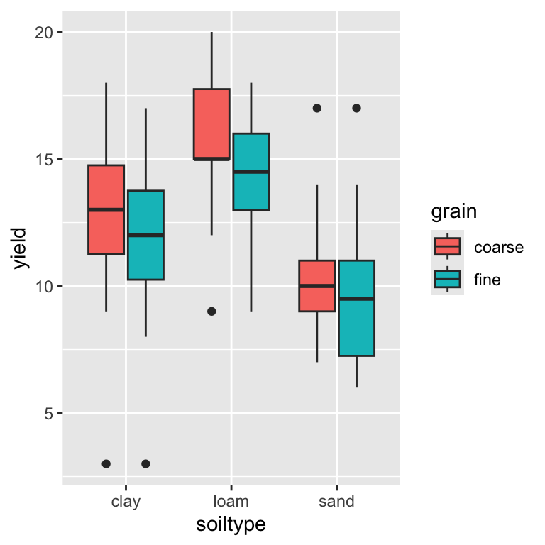
Pipes
Data wrangling often involves several transformation steps that build on one another. To write code that clearly reflects this step-by-step logic, the dplyr package provides pipes, which allow you to chain operations together in a readable sequence. With pipes, an expression like x |> f(y) is interpreted as f(x, y), making it easier to follow the flow of data through each transformation. The base R pipe (|>) and the dplyr pipe (%>%) serve similar purposes, but the dplyr pipe offers additional conveniences.
yields2_tidy <- yields2 %>%
  pivot_longer(cols= -plotid, names_to = "soiltype", values_to = "yield") %>%
  separate(col = soiltype, into = c("soiltype", "grain"), sep = "_")
Mutating new variables
If we want to create a new variable (column), we can use the mutate() function:
yields2_tidy <- yields2_tidy %>%
  mutate(yield_log = log(yield),
         yield_log10 = log10(yield))

yields2_tidy[1:3, ]
# A tibble: 3 × 6
plotid soiltype grain yield yield_log yield_log10
<int> <chr> <chr> <int> <dbl> <dbl>
1 1 sand fine 6 1.79 0.778
2 1 clay fine 17 2.83 1.23
3 1 loam fine 13 2.56 1.11 Summaries
If we want to create a summary of (a) variable(s), we can use the summarize() function:
yields2_tidy_summary <- yields2_tidy %>%
  summarize(yield_mean = mean(yield),
            yield_median = median(yield))

yields2_tidy_summary
# A tibble: 1 × 2
yield_mean yield_median
<dbl> <dbl>
1 12.4 12Grouping
Using dyplr we can easily calculate new variables or derive summaries of our data. However, often we want to do both wihtin specific groups, e.g. the mean/median yield within each soil-type and grain-class. We therefore need to group the data:
yields2_tidy_summary <- yields2_tidy %>%
  group_by(soiltype, grain) %>%
  summarize(yield_mean = mean(yield),
            yield_median = median(yield))
`summarise()` has grouped output by 'soiltype'. You can override using the
`.groups` argument.yields2_tidy_summary# A tibble: 6 × 4
# Groups: soiltype [3]
soiltype grain yield_mean yield_median
<chr> <chr> <dbl> <dbl>
1 clay coarse 12.4 13
2 clay fine 11.5 12
3 loam coarse 15.5 15
4 loam fine 14.3 14.5
5 sand coarse 10.6 10
6 sand fine 9.9 9.5We also can use the mutate() function within groups, e.g. for centering the yields within groups:
yields2_tidy <- yields2_tidy %>%
  group_by(soiltype, grain) %>%
  mutate(yield_centered = yield - mean(yield))

yields2_tidy
# A tibble: 60 × 7
# Groups: soiltype, grain [6]
plotid soiltype grain yield yield_log yield_log10 yield_centered
<int> <chr> <chr> <int> <dbl> <dbl> <dbl>
1 1 sand fine 6 1.79 0.778 -3.9
2 1 clay fine 17 2.83 1.23 5.5
3 1 loam fine 13 2.56 1.11 -1.3
4 1 sand coarse 9 2.20 0.954 -1.6
5 1 clay coarse 18 2.89 1.26 5.6
6 1 loam coarse 15 2.71 1.18 -0.5
7 2 sand fine 10 2.30 1 0.1000
8 2 clay fine 15 2.71 1.18 3.5
9 2 loam fine 16 2.77 1.20 1.7
10 2 sand coarse 10 2.30 1 -0.600
# ℹ 50 more rowsTibbles
Note: The result from a dplyr call is a so-called tibble, which is similar to a data frame, but has some improvements. For example, it shows the data type and dimensions of the data frame, as well as it is easier to print in the console.
head(yields_tidy)# A tibble: 6 × 3
plotid soiltype yield
<int> <chr> <int>
1 1 sand 6
2 1 clay 17
3 1 loam 13
4 2 sand 10
5 2 clay 15
6 2 loam 16Subsetting data
Often, we also want to exclude observations (rows), which we can easily do using the filter() function:
yields2_tidy_subset <- yields2_tidy %>%
  filter(grain == "fine")
Similarly, we can exclude variables (columns) that we don’t need for further analysis using the select() function:
yields2_tidy_subset <- yields2_tidy %>%
  select(-yield_log10, -yield_log)
Thereby we ca either select columns or drop them using a ‘-’ before the columns name.