library(terra)
library(ggplot2)
library(cowplot)12 Tasseled cap
Packages
Bits explained
Computers internally represent integers as bits. A single bit can store two values: 1 or 0, which you may interpret as on or off. If you want to store more values, you need more bits. For example, with 8 bits you can store 256 integer values, i.e., there are \(2^8\) ways to combine 8 bits. Below is a sketch of 8 bits. We count the bits from right to left. The right-most bit is bit 0 and the left-most bit is bit 7. Here, only bit 1 and bit 2 are on.
Bit string   :   0  0  0  0 0 1 1 0
Bit number   :   7  6  5  4 3 2 1 0
Integer value: 128 64 32 16 8 4 2 1
Each bit has a specific integer value. Bit 0 has the integer value \(2^0=1\), bit 1 has the integer value \(2^1=2\), bit 2 has the integer value \(2^2=4\), bit 3 has the integer value \(2^3=8\), and so forth.
2^(7:0)[1] 128 64 32 16 8 4 2 1The example above, with bit 1 and bit 2 set to 1, corresponds to an integer value of \(2^1 + 2^2 = 6\). We can check this by casting the integer back into a bit representation. Note that intToBits() places the least significant bit on the left, returns a vector of raw bytes rather than characters, and prints these bytes in hexadecimal using two digits. Applying rev() reverses the order of the bits, and as.integer() converts the raw values to 0s and 1s.
as.integer(rev(intToBits(6))) [1] 0 0 0 0 0 0 0 0 0 0 0 0 0 0 0 0 0 0 0 0 0 0 0 0 0 0 0 0 0 1 1 0With 8 bits we can represent all integer values from 0 to 255. The maximum value is obtained by summing the contributions of all bits when they are set to 1.
sum(2^(7:0))[1] 255With 16 bits, we can encode 65535 values, i.e., either from 0 to 65535 or -32767 to 32767.
sum(2^(15:0))[1] 65535Bit masking
Bit strings are sometimes used to encode multiple values or conditions. For example, bit 1 may represent one condition, while bit 2 represents another. The Landsat cloud mask is one example of this approach. To determine whether a particular condition is true, we check whether the corresponding bit is set. This is done using a bitwise operation, a process often referred to as bit masking.
Specifically, bitwAnd() performs a bitwise AND operation, keeping only the bits that are set in both its arguments. It can be used to isolate the bits corresponding to a particular mask.
For example, consider our bit string representing the integer 6 (binary 0110). If we apply a mask for bit 1, which corresponds to integer 2 (binary 0010), bitwAnd(6, 2) returns 2, indicating that bit 1 is set in the original number.
bitwAnd(6, 2)[1] 2In a bitwise (bit-by-bit) AND operation, the bits on the left represent the original number, and the bits on the right represent the mask. Each pair of corresponding bits is combined according to the AND rules:
0 AND 0 = 01 AND 1 = 11 AND 0 = 00 AND 0 = 00 AND 0 = 00 AND 0 = 00 AND 0 = 00 AND 0 = 0
The result is a new bit string where only the bits that are set in both the original number and the mask remain 1; all other bits become 0.
Bit 1 contributes to several integers, such as 2, 3, 6, 7, and so on. Therefore, bitwAnd(x, 2) will return 2 for any of these integers. You can try this yourself:
- The integer
3has both bit 0 and bit 1 set. Hence,bitwAnd(3, 2)returns2. - The integer
2has only bit 1 set, sobitwAnd(2, 2)returns2. - The integer
1has only bit 0 set, sobitwAnd(1, 2)returns0.
Note
It can be useful and convenient to shift bits before extracting them. For example, shifting the bit string to the right by 1 position puts bit 1 in the position of bit 0. We can then extract the former bit 1 at position 0 as we did before, e.g. bitwAnd(bitwShiftR(6, 1), 1) will return 1.
Landsat data
Landsat data are provided by the United States Geological Survey (USGS) in different processing levels, tiers, and collections. Collections represent the major versions of the entire Landsat processing pipeline, including the radiometric and geometry processing. In early 2021, Landsat Collection 2 was released with improved processing, geometric accuracy, and radiometric calibration compared to previous Collection 1 products. Tiers are categories that signify the processing grade and accuracy. Among the three available tiers, only Tier 1 is going to be relevant for us. It has the highest radiometric and positional quality. Finally, levels signify the type and amount of processing one or multiple scenes received. In this course, we are using Landsat Level-2 data. Level-2 data were processed to surface reflectance using atmospheric correction algorithms and they also contain cloud masks. Surface reflectance allows a comparison between multiple images over the same region by accounting for atmospheric effects such as aerosol scattering and thin clouds. Surface reflectance is calculated for every image that was acquired with less than 76° solar zenith angle and has the required auxiliary data inputs (see Landsat Science Product Guide).
A single Landsat Collection-2 Level-2 scene consists of a number of files, specifically surface reflectance bands (SR), surface temperature bands (ST), and a number of quality assurance bands (Table 12.1). In Table 12.1 we can also see that the surface reflectance bands are stored as unsigned 16-bit integers, that the fill value (nodata value) is 0, and that the data was scaled with a multiplicative scale factor and an additive offset (Section 12.3.3).
| Band Designation | Band Name | Data Type | Units | Data Range | Valid Range | Fill Value | Scale Factor | Offset |
|---|---|---|---|---|---|---|---|---|
| ProductID_SR_B1 | Band 1 SR | UINT16 | Reflectance | 1 - 65535 | 7273 - 43636 | 0 | 0.0000275 | -0.2 |
| ProductID_SR_B2 | Band 2 SR | UINT16 | Reflectance | 1 - 65535 | 7273 - 43636 | 0 | 0.0000275 | -0.2 |
| ProductID_SR_B3 | Band 3 SR | UINT16 | Reflectance | 1 - 65535 | 7273 - 43636 | 0 | 0.0000275 | -0.2 |
| ProductID_SR_B4 | Band 4 SR | UINT16 | Reflectance | 1 - 65535 | 7273 - 43636 | 0 | 0.0000275 | -0.2 |
| ProductID_SR_B5 | Band 5 SR | UINT16 | Reflectance | 1 - 65535 | 7273 - 43636 | 0 | 0.0000275 | -0.2 |
| ProductID_SR_B6 | Band 6 SR | UINT16 | Reflectance | 1 - 65535 | 7273 - 43636 | 0 | 0.0000275 | -0.2 |
| ProductID_SR_B7 | Band 7 SR | UINT16 | Reflectance | 1 - 65535 | 7273 - 43636 | 0 | 0.0000275 | -0.2 |
| ProductID_ST_B10 | Band 10 ST | UINT16 | Kelvin | 1 - 65535 | 293 - 61440 | 0 | 0.0034180 | 149.0 |
| ProductID_QA_PIXEL | Level 2 Pixel Quality Band | UINT16 | Bit Index | 1 - 65535 | 21824 - 65534 | 1 | NA | NA |
| ProductID_SR_QA_AEROSOL | Aerosol QA | UINT8 | Bit Index | 0 - 255 | 1 - 255 | 1 | NA | NA |
| ProductID_QA_RADSAT | Radiometric Saturation QA | UINT16 | Bit Index | 0 - 65535 | 0 - 3829 | NA | NA | NA |
| ProductID_ST_QA | Surface Temperature Uncertainty | INT16 | Kelvin | 0 - 32767 | 0 - 32767 | -9999 | 0.0100000 | NA |
| ProductID_ST_TRAD | Thermal Radiance | INT16 | W/(m^{2} .sr._m)/ DN | 0 - 22000 | 0 - 22000 | -9999 | 0.0010000 | NA |
| ProductID_ST_URAD | Upwelled Radiance | INT16 | W/(m^{2} .sr._m)/ DN | 0 - 28000 | 0 - 28000 | -9999 | 0.0010000 | NA |
| ProductID_ST_DRAD | Downwelled Radiance | INT16 | W/(m^{2} .sr._m)/ DN | 0 - 28000 | 0 - 28000 | -9999 | 0.0010000 | NA |
| ProductID_ST_ATRAN | Atmospheric Transmittance | INT16 | Unitless | 0 - 10000 | 0 - 10000 | -9999 | 0.0001000 | NA |
| ProductID_ST_EMIS | Emissivity estimated from ASTER GED | INT16 | Unitless | 0 - 10000 | 0 - 10000 | -9999 | 0.0001000 | NA |
| ProductID_ST_EMSD | Emissivity standard deviation | INT16 | Unitless | 0 - 32767 | 0 - 10000 | -9999 | 0.0001000 | NA |
| ProductID_ST_CDIST | Pixel distance to cloud | INT16 | Kilometers | 0 - 24000 | 0 - 24000 | -9999 | 0.0100000 | NA |
| ProductID_MTL | Level 2 Metadata file | NA | NA | NA | NA | NA | NA | NA |
Download
You can search and download Landsat Level-2 surface reflectance data from the EarthExplorer or or the Global Visualization Viewer (GloVis). The USGS provides an overview on how to get Landsat data see here.
Read Landsat data
Landsat’s spectral bands and quality bands come in separate GeoTIFF files (Table 12.1). The spectral bands most relevant for land surface analysis are Bands 2-7. To read them into R, we first need to create a list of the corresponding file names (actually a character vector - not a list). The list.files() function lets us do this automatically. The function takes a directory name and a search pattern as input argument. We want to find all files in the image directory that contain the characters SR_B. The pattern argument takes a regular expression, which is a powerful but also complex language (sort of). The function glob2rx() lets us specify a wildcard (*) pattern and turns it into a regular expression. The wildcard matches any kind of character or string.
l8_bands <- list.files("data/landcov/LC08_L2SP_193023_20170602_20200903_02_T1/",
                       pattern = glob2rx("*SR_B*TIF"),
                       full.names = TRUE)
l8_bands
[1] "data/landcov/LC08_L2SP_193023_20170602_20200903_02_T1//LC08_L2SP_193023_20170602_20200903_02_T1_SR_B1.TIF"
[2] "data/landcov/LC08_L2SP_193023_20170602_20200903_02_T1//LC08_L2SP_193023_20170602_20200903_02_T1_SR_B2.TIF"
[3] "data/landcov/LC08_L2SP_193023_20170602_20200903_02_T1//LC08_L2SP_193023_20170602_20200903_02_T1_SR_B3.TIF"
[4] "data/landcov/LC08_L2SP_193023_20170602_20200903_02_T1//LC08_L2SP_193023_20170602_20200903_02_T1_SR_B4.TIF"
[5] "data/landcov/LC08_L2SP_193023_20170602_20200903_02_T1//LC08_L2SP_193023_20170602_20200903_02_T1_SR_B5.TIF"
[6] "data/landcov/LC08_L2SP_193023_20170602_20200903_02_T1//LC08_L2SP_193023_20170602_20200903_02_T1_SR_B6.TIF"
[7] "data/landcov/LC08_L2SP_193023_20170602_20200903_02_T1//LC08_L2SP_193023_20170602_20200903_02_T1_SR_B7.TIF"We can read the individual Landsat bands as a single, multiband image (SpatRaster) using the rast() function from the terra package. Raster layers can be combined from different files as long as the layers match in extent and resolution. Note, we are excluding the aerosol Band 1 with l8_bands[-1].
l8img <- rast(l8_bands[-1])
l8img
class : SpatRaster
size : 8141, 8051, 6 (nrow, ncol, nlyr)
resolution : 30, 30 (x, y)
extent : 278085, 519615, 5762085, 6006315 (xmin, xmax, ymin, ymax)
coord. ref. : WGS 84 / UTM zone 33N (EPSG:32633)
sources : LC08_L2SP_193023_20170602_20200903_02_T1_SR_B2.TIF
LC08_L2SP_193023_20170602_20200903_02_T1_SR_B3.TIF
LC08_L2SP_193023_20170602_20200903_02_T1_SR_B4.TIF
... and 3 more sources
names : LC08_~SR_B2, LC08_~SR_B3, LC08_~SR_B4, LC08_~SR_B5, LC08_~SR_B6, LC08_~SR_B7 It’s always a good idea to assign short but meaningful band names.
names(l8img) <- paste0("B", 2:7)
l8img
class : SpatRaster
size : 8141, 8051, 6 (nrow, ncol, nlyr)
resolution : 30, 30 (x, y)
extent : 278085, 519615, 5762085, 6006315 (xmin, xmax, ymin, ymax)
coord. ref. : WGS 84 / UTM zone 33N (EPSG:32633)
sources : LC08_L2SP_193023_20170602_20200903_02_T1_SR_B2.TIF
LC08_L2SP_193023_20170602_20200903_02_T1_SR_B3.TIF
LC08_L2SP_193023_20170602_20200903_02_T1_SR_B4.TIF
... and 3 more sources
names : B2, B3, B4, B5, B6, B7 Recall, we can display a color composite using plotRGB().
plotRGB(l8img, r = 3, g = 2, b = 1, stretch = "hist")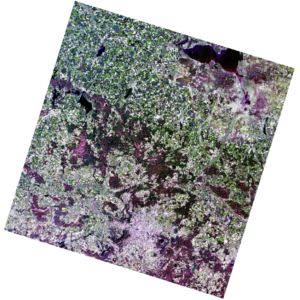
Scaling
The Landsat surface reflectance data are in unsigned 16-bit integers (0 to 65535). Integers are whole numbers, and unsigned means only positive whole numbers. Originally, surface reflectance values (\(\rho\)) are fractions (decimal numbers) ranging from 0 to 1. Since, decimal numbers can only be stored as 32-bit floating point values (or higher), scaling the decimals to integers saves space (e.g., half the file size).
To convert a decimal number to an integer usually requires that we scale (multiply) the decimal number by some value. For example, we could multiply the fractions by the scalar 100 and convert the results to integers. This way we would retain a level of precision of 0.01 reflectance units. Using a multiplier of 10,000 would retain a precision of 0.0001 reflectance units. To convert back to reflectance we would need to multiply the integer by 0.01 (1/100) or 0.0001 (1/10,000), respectively. We can formulate this as an equation:
\[ \rho = gain*DN + offset \tag{12.1}\]
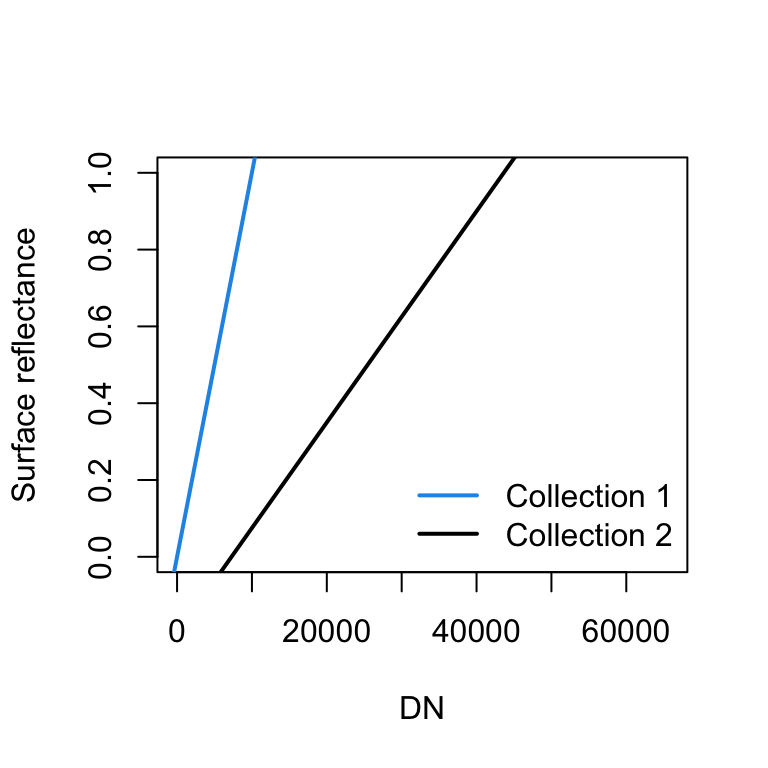
where, \(\rho\) is reflectance, \(DN\) are the integer digital numbers, \(gain\) is our multiplicative scale factor (e.g., 0.0001) and \(offset\) is an additive scale value. We did not define an offset in our example above, so offset was zero. In fact, the USGS used an offset of zero and a gain of 0.0001 in collection 1. In collection 2, the USGS changed the gain to 0.0000275 and introduced an additive offset of -0.2 to further increase precision.
Let’s apply the scale and offset to convert the Landsat image pixel values to surface reflectance.
l8img <- l8img * 0.0000275 - 0.2
Warning
You must rescale Landsat Collection 2 data to reflectance before calculating vegetation indices or other transformations. While multiplicative scaling does not change such indices, the additive offset does.
The scaling Equation 12.1 is a linear function. We can plot the linear function corresponding to collection 1 and collection 2. Notice that collection 2 maps the reflectance to a wider range of integers (DN), and thus achieves a higher level of precision.
Cloud masking
Landsat Surface Reflectance products include Quality Assessment (QA) bands to flag pixels affected by instrument, atmospheric, or surface conditions. The QA_PIXEL band encodes information at the pixel level regarding fill (no data), clouds, cloud shadows, snow/ice, water, and confidence levels for clouds, cloud shadows, snow/ice, and cirrus.
qa_pixel <- rast(file.path(
                  "data/landcov/LC08_L2SP_193023_20170602_20200903_02_T1/",
                  "LC08_L2SP_193023_20170602_20200903_02_T1_QA_PIXEL.TIF"))

unique(values(qa_pixel))[,1]
[1] 1 21824 22080 22280 21952 23888 21762 22018 23826 24144 24082 21890 22208 54596 54724 55052
[17] 56598 54534 54662 56660 54852 54790 56854 56916 62820 62758 30048The QA_PIXEL band contains integer values, but unlike a land cover map, the quality conditions are not represented by distinct integer codes. Instead, individual quality conditions are encoded at the bit level. If you have not read Section 12.2, now this is a good time to learn about the connection between bits and integers. Table 12.2 lists the bit-coding and Table 12.3 the associated integer values from QA_PIXEL (see also Science Product Guide).
| Bit | Flag Description | Values |
|---|---|---|
| 0 | Fill | 0 for image data 1 for fill data |
| 1 | Dilated Cloud | 0 for cloud is not dilated or no cloud 1 for cloud dilation |
| 2 | Cirrus | 0 for Cirrus Confidence: no confidence level set or Low Confidence 1 for high confidence cirrus |
| 3 | Cloud | 0 for cloud confidence is not high 1 for high confidence cloud |
| 4 | Cloud Shadow | 0 for Cloud Shadow Confidence is not high 1 for high confidence cloud shadow |
| 5 | Snow | 0 for Snow/Ice Confidence is not high 1 for high confidence snow cover |
| 6 | Clear | 0 if Cloud or Dilated Cloud bits are set 1 if Cloud and Dilated Cloud bits are not set |
| 7 | Water | 0 for land or cloud 1 for water |
| 8-9 | Cloud Confidence | 00 for no confidence level set 01 Low confidence 10 Medium confidence 11 High confidence |
| 10-11 | Cloud Shadow Confidence | 00 for no confidence level set 01 Low confidence 10 Reserved 11 High confidence |
| 12-13 | Snow/Ice Confidence | 00 for no confidence level set 01 Low confidence 10 Reserved 11 High confidence |
| 14-15 | Cirrus Confidence | 00 for no confidence level set 01 Low confidence 10 Reserved 11 High confidence |
| Pixel Value | Fill | Dilated Cloud | Cirrus | Cloud | Cloud Shadow | Snow | Clear | Water | Cloud Conf. | Cloud Shadow.Conf. | Snow .Ice.Conf. | Cirrus Conf. | Pixel Description |
|---|---|---|---|---|---|---|---|---|---|---|---|---|---|
| 1 | Yes | No | No | No | No | No | No | No | None | None | None | None | Fill |
| 21824 | No | No | No | No | No | No | Yes | No | Low | Low | Low | Low | Clear with lows set |
| 21826 | No | Yes | No | No | No | No | Yes | No | Low | Low | Low | Low | Dilated cloud over land |
| 21888 | No | No | No | No | No | No | No | Yes | Low | Low | Low | Low | Water with lows set |
| 21890 | No | Yes | No | No | No | No | No | Yes | Low | Low | Low | Low | Dilated cloud over water |
| 22080 | No | No | No | No | No | No | Yes | No | Mid | Low | Low | Low | Mid conf cloud |
| 22144 | No | No | No | No | No | No | No | Yes | Mid | Low | Low | Low | Mid conf cloud over water |
| 22280 | No | No | No | Yes | No | No | No | No | High | Low | Low | Low | High conf Cloud |
| 23888 | No | No | No | No | Yes | No | Yes | No | Low | High | Low | Low | High conf cloud shadow |
| 23952 | No | No | No | No | Yes | No | No | Yes | Low | High | Low | Low | Water with cloud shadow |
| 24088 | No | No | No | Yes | Yes | No | No | No | Mid | High | Low | Low | Mid conf cloud with shadow |
| 24216 | No | No | No | Yes | Yes | No | No | Yes | Mid | High | Low | Low | Mid conf cloud with shadow over water |
| 24344 | No | No | No | Yes | Yes | No | No | No | High | High | Low | Low | High conf cloud with shadow |
| 24472 | No | No | No | Yes | Yes | No | No | Yes | High | High | Low | Low | High conf cloud with shadow over water |
| 30048 | No | No | No | No | No | Yes | Yes | No | Low | Low | High | Low | High conf snow/ice |
| 54596 | No | No | Yes | No | No | No | Yes | No | Low | Low | Low | High | High conf Cirrus |
| 54852 | No | No | Yes | No | No | No | Yes | No | Mid | Low | Low | High | Cirrus; mid cloud |
| 55052 | No | No | Yes | Yes | No | No | No | No | High | Low | Low | High | Cirrus; high cloud |
| 56856 | No | No | No | Yes | Yes | No | No | No | Mid | High | Low | High | Cirrus; mid conf cloud; shadow |
| 56984 | No | No | No | Yes | Yes | No | No | Yes | Mid | High | Low | High | Cirrus; mid conf cloud; shadow; over water |
| 57240 | No | No | No | Yes | Yes | No | No | Yes | High | High | Low | High | Cirrus; high conf cloud; shadow |
Technically, there are two ways to extract a mask of clear observations: 1) based on bitwise operations that extract specific bits (conditions) as in Table 12.2, and 2) based on the integer values associated with the quality conditions in Table 12.3 (not recommended). The sketch below illustrates the connection between the Landsat QA bits and their integer representation.
![]()
Integer mask
Create a mask for clear and water pixels based on the integer values that correspond to these conditions (Table 12.3). To evaluate against multiple values, you may use %in%. However, this method is not recommended. Experience shows that the integer values listed in the table may be incomplete.
l8mask1 <- qa_pixel %in% c(21824, 21888, 21952, 30048)
plot(l8mask1)
Bit mask
We can use bitwise AND (Section 12.2) to check (mask) the bits that correspond to specific QA conditions Table 12.2. Specifically, we want to isolate three bits: bit 5 (snow), bit 6 (clear land), and bit 7 (water). To extract bit 6, we can do bitwAnd(b, 64), because bit 6 corresponds to integer 64 (\(2^6=64\)). In our case, we want to flag all pixels where any these three bits is set. The function is_valid() implements this logic and returns TRUE if a pixel is flagged as snow, clear land or water. Each bitwAnd() call returns a non-zero integer when the corresponding bit is on. These results are combined with the logical OR operator |, which treats non-zero values as TRUE and zero as FALSE.
To apply this function to the entire quality band, we can use app() from the terra package.
is_valid <- function(x) { (bitwAnd(x, 32) |
                           bitwAnd(x, 64) |
                           bitwAnd(x, 128) )}

l8mask <- app(qa_pixel, fun=is_valid)

plot(l8mask)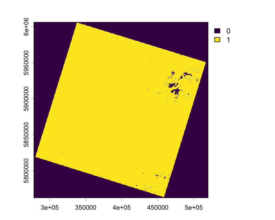
Note
Alternatively, you can mask all three bits in one operation using the integer mask 224 (32 + 64 + 128 = 224). The function bitwAnd(x, 224) returns a non-zero integer if any of the three bits are set. To return a binary mask you need to compare it against zero: bitwAnd(x, 224) != 0.
Mask image
The l8mask image now contains 1s (TRUE) for clear pixels and 0s (FALSE) for everything else (cloud/shadow/fill). We can apply this binary mask to the Landsat-8 image, replacing non-valid pixels with NA (this may take few minutes):
l8img_masked <- terra::mask(l8img, l8mask, maskvalues = 0)

plotRGB(l8img_masked, r = 3, g = 2, b = 1, stretch = "hist")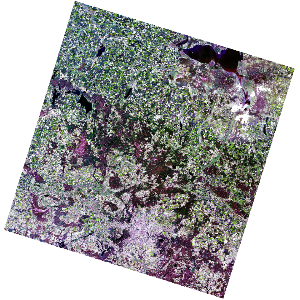
Zoom and crop
Select a subset of the image. You can use the zoom() function to find an area that you like. Choose an area that has a mix of different land cover types. The zoom() function returns a SpatExtent object (bounding box) and adds a new zoom plot to the plot window.
berlinExtent <- zoom(l8img_masked)
berlinExtent
SpatExtent : 359070, 413150, 5797900, 5845260 (xmin, xmax, ymin, ymax)
Note
The function zoom() works only in the interactive console. You cannot use it in markdown documents. In RStudio, you must change the settings (next to the knit button) to Chunk Output in Console. For your assignment, you need to create the SpatExtent object manually, using the coordinates returned by zoom().
berlinExtent <- ext(c(359070, 413150, 5797900, 5845260))You can use the SpatExtent object to crop the image to the selected area (Figure 12.3).
l8img_subset <- crop(l8img_masked, berlinExtent)
plotRGB(l8img_subset, r = 3, g = 2, b = 1, stretch = "hist")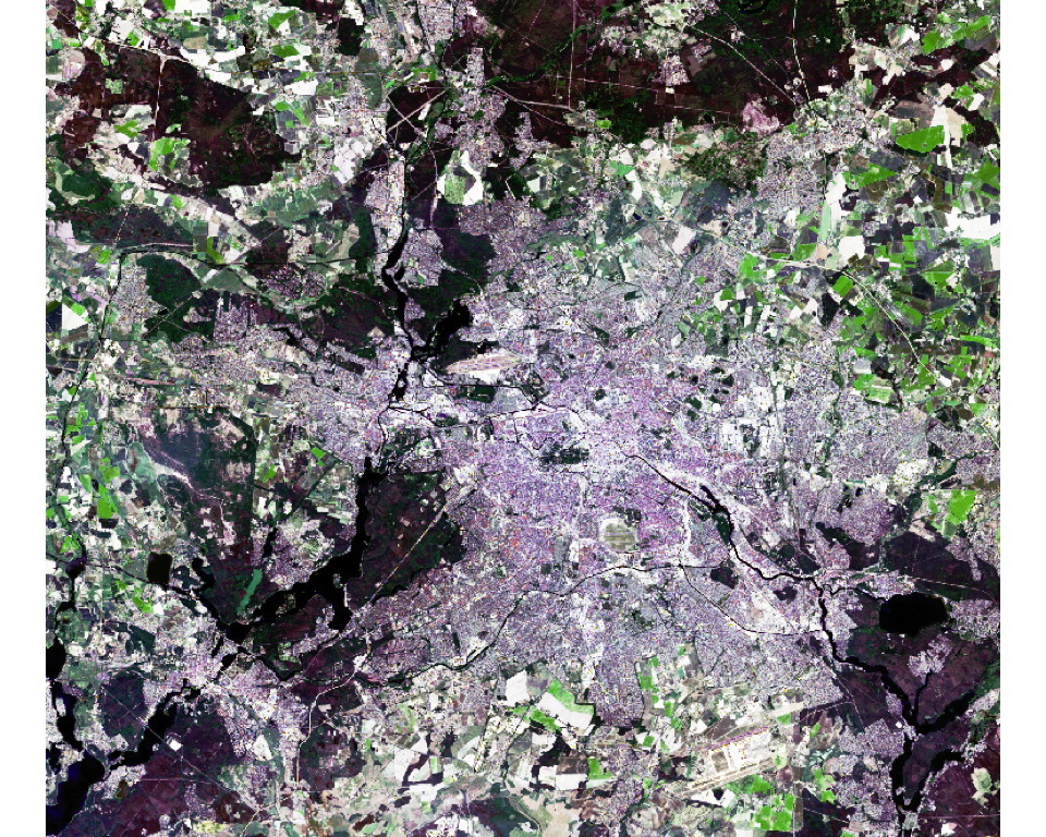
writeRaster(l8img_subset2, 'data/landcov/LC08_L2SP_193023_20170602_20200903_02_T1_sr_cropped.tif', format='GTiff', overwrite=T)Transformations
Spectral bands are often highly correlated with each other and do not directly correspond to the environmental feature of interest (e.g., vegetation greenness, soil moisture). Confounding factors, such as soil background and illumination differences can further obscure meaningful patterns. Transformations, such as band ratios, vegetation indices, principal component analyses, or the Tasseled Cap transformation, are applied to:
- reduce redundancy,
- minimize the influence of confounding variables, and
- enhance the signal relevant to the phenomenon of interest.
Show code
# Sample Landsat data
l8sample <- spatSample(l8img, size = 100000, na.rm=T)

# Plot 1: Blue vs Green
p1 <- ggplot(l8sample, aes(x = B2, y = B3)) +
  geom_hex(binwidth = 0.01) +
  geom_smooth(method = "lm", color = "red", se = FALSE, linewidth = 0.5) +
  xlab("Blue") + ylab("Green") +
  xlim(0, 0.7) + ylim(0, 0.7) +
  scale_fill_continuous(type = "viridis") +
  theme_classic() +
  theme(legend.position = "none")

# Plot 2: Red vs NIR
p2 <- ggplot(l8sample, aes(x = B4, y = B5)) +
  geom_hex(binwidth = 0.01) +
  geom_smooth(method = "lm", color = "red", se = FALSE, linewidth = 0.5) +
  xlab("Red") + ylab("NIR") +
  xlim(0, 0.7) + ylim(0, 0.7) +
  scale_fill_continuous(type = "viridis") +
  theme_classic() +
  theme(legend.position = "none")

# Plot side by side
plot_grid(p1, p2, ncol = 2)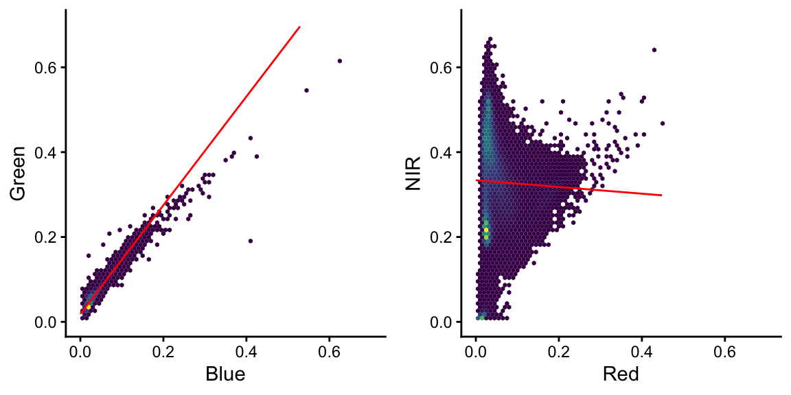
Tasseled cap
The tasseled cap transformation is a linear transformation of multispectral satellite data designed to highlight key features of the land surface. It converts the original spectral bands into new components (brightness, greenness, and wetness) that represent soil reflectance, vegetation vigor, and moisture/structure conditions, respectively. This transformation simplifies the analysis of vegetation and land cover dynamics and is widely used with sensors such as Landsat and Sentinel-2 for monitoring environmental change.
A linear transformation means that each tasseled cap component is calculated as a weighted sum of the individual satellite bands, where the weights are defined by the tasseled cap coefficients. For example, we can calculate \(brightness\) as:
\[ brightness = 0.2043 * band_{blue} + 0.4158 * band_{green} + ... + 0.2303 * band_{swir2} \]
A more general formulation for each component \(i\) is:
\[ component_i = \sum_{j=1}^{6} \beta_{i,j} * band_j \]
where the \(\beta\)’s are the coefficients for the \(i\)’s component (e.g. brightness, greenness, wetness) and the \(j\)’s are Landsat bands.
In this class, we use the coefficients from Crist (1985), which were derived for Landsat TM surface reflectance data (Table 12.4). Although coefficients for more recent sensors have been published, many of them are based on top-of-atmosphere reflectance rather than surface reflectance. In practice, tasseled cap transformations are often applied to time series that combine data from multiple sensors. For this reason, it is generally more important to use a consistent single set of coefficients to avoid introducing potential biases, rather than switching between sensor-specific versions. Furthermore, since none of the existing coefficient sets were developed for truly global datasets, using a well-established and widely tested set such as Crist’s remains a sound and practical choice.
| Blue | Green | Red | NIR | SWIR1 | SWIR2 | |
|---|---|---|---|---|---|---|
| Brightness | 0.2043 | 0.4158 | 0.5524 | 0.5741 | 0.3124 | 0.2303 |
| Greenness | -0.1603 | -0.2819 | -0.4934 | 0.7940 | -0.0002 | -0.1446 |
| Wetneess | 0.0315 | 0.2021 | 0.3102 | 0.1594 | -0.6806 | -0.6109 |
Note
Using the coefficients provided below, you can calculate each tasseled cap component in R with simple raster math operations.
coeffs <- matrix(c( 0.2043,  0.4158,  0.5524, 0.5741,  0.3124,  0.2303,
                   -0.1603, -0.2819, -0.4934, 0.7940, -0.0002, -0.1446,
                    0.0315,  0.2021,  0.3102, 0.1594, -0.6806, -0.6109),
                 nrow = 3, byrow = TRUE)
row.names(coeffs) <- c("brightness", "greenness", "wetness")
coeffs
[,1] [,2] [,3] [,4] [,5] [,6]
brightness 0.2043 0.4158 0.5524 0.5741 0.3124 0.2303
greenness -0.1603 -0.2819 -0.4934 0.7940 -0.0002 -0.1446
wetness 0.0315 0.2021 0.3102 0.1594 -0.6806 -0.6109