Code
library(lubridate) # manipulation of date and time
library(ggplot2)   # graphics
library(tidyr) # manipulation of data.frameslibrary(lubridate) # manipulation of date and time
library(ggplot2) # graphics
library(tidyr) # manipulation of data.framesDealing with coding errors is a complex topic. Fortunately, there are a number of good tools and documentation available for R (e.g., Wickham (2019), Chapter Conditions and Debugging). We are not covering the topic in detail here. But we will focus on a specific use case.
The function tryCatch() is useful when you expect an (occasional) error, but rather than stopping the program, you want to handle the error automatically. For example, a function that computes a statistic on a vector may fail in certain conditions, e.g., if there are too few observations. Let’s look at a simple example. The function square() takes a single argument as input and squares it. If the argument is not of type numeric, then the function throws an error and your program stops.
square<- function(x) x^2
square("2")
Error in x^2: non-numeric argument to binary operatorWhen we put the function inside tryCatch(), we can define a function that is triggered when an error occurs. In the case below, the function would return NA. This is a simple example, which we could handle more directly, e.g., by converting the character string into a numeric. But there are cases, when you are not able to fix the error but still want the function to return something.
a <- "2"
tryCatch(
  error=function(e) return(NA),
  square(a)
)
[1] NAUse tryCatch() with caution. You might be tempted to apply it in many situations. However, an error is an indication that something is wrong. Blindly ignoring the error will jeopardize your analysis.
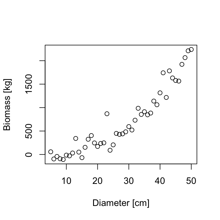
In the course so far, we’ve used linear models to describe the relationship between variables and, when necessary, we’ve used transformations to linearize that relationship. However, sometimes a linear model is not an adequate choice. In this case, we might use a non-linear regression model. Typically, we have some idea of the functional relationship between two variables based on prior knowledge of the data or underlying mechanisms. For example, the relationship between tree biomass \(B\) and tree diameter \(D\) may be described with a power function:
\[B=\alpha*D^{\beta} \tag{18.1}\]
Based on our power function, we can estimate the non-linear parameters \(\alpha\) and \(\beta\) using nls(). The function nls() takes a formula as input, but unlike lm() and glm(), the model formula for nls() does not use the special codings for linear terms and interactions. Instead, we write an explicit expression of the curve that we are trying to fit:
bmod <- nls(B ~ a*D^b, data=tree, start=?)Just based on the formula, it is not clear (to R) which letter represents a variable (\(B\) and \(D\)) and which a parameter (\(a\) and \(b\)). So we need to specify which is which. Specifically, we specify the parameter names and their starting values with the start argument. The start argument takes a data.frame, a named vector, or a list. We need to define starting values, because there is no algebraic solution for minimizing the least-squares with non-linear models (as there is with linear models). Non-linear models find the least-squares fit by solving an optimization problem, which requires a (reasonably good) staring estimate.
bmod <- nls(B ~ a*D^b, data=tree, start=c(a=0.5, b=2))
summary(bmod)
Formula: B ~ a * D^b

Parameters:
  Estimate Std. Error t value Pr(>|t|)
a  0.10684    0.06011   1.777   0.0824 .
b  2.54314    0.14959  17.000   <2e-16 ***
---
Signif. codes:  0 '***' 0.001 '**' 0.01 '*' 0.05 '.' 0.1 ' ' 1

Residual standard error: 162.2 on 44 degrees of freedom

Number of iterations to convergence: 7
Achieved convergence tolerance: 7.884e-07
We can extract the parameters with the coef() function:
params <- coef(bmod)
params
a b
0.1068419 2.5431432 The non-linear model estimates \(\alpha=0.10684\) and \(\beta=2.54314\). Replacing the estimates in the power function formula, we can plot the resulting curve.
plot(B ~ D, data=tree)
curve(params['a']*x^params['b'], from=5, to=50, add=T, col=4, lwd=2)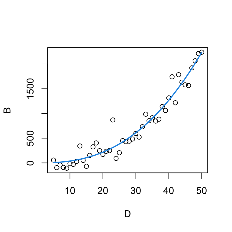
Here, the ggplot version of the graph above (without plotting the graph).
ggplot(tree, aes(x=D, y=B)) +
  geom_point() +
geom_function(fun = function(x) params['a']*x^params['b'], colour = "blue")The MODIS sensor on-board the Terra and Aqua satellites has been providing near daily observations of the entire globe since 2000. For this exercise, we will use the MODIS vegetation index product (MOD13Q1). The product provides 16-day composites of the vegetation indices NDVI and EVI for the Terra (MOD) and Aqua (MYD) platform, respectively. Combining Terra and Aqua gives us a time interval of 8-days. See the product guide for more detailed information. Each 16-day product contains the following layers. The pixel reliability layer ranks pixels according to their quality.
| ScienceData Set | Units | Data type | Valid Range | Scale factor |
|---|---|---|---|---|
| 16 days NDVI | NDVI | int16 | -2000, 10000 | 0.0001 |
| 16 days EVI | EVI | int16 | -2000, 10000 | 0.0001 |
| 16 days VI Quality detailed QA | Bits | uint16 | 0, 65534 | NA |
| 16 days red reflectance (Band 1) | Reflectance | int16 | 0, 10000 | 0.0001 |
| 16 days NIR reflectance (Band 2) | Reflectance | int16 | 0, 10000 | 0.0001 |
| 16 days blue reflectance (Band 3) | Reflectance | int16 | 0, 10000 | 0.0001 |
| 16 days MIR reflectance (Band 7) | Reflectance | int16 | 0, 10000 | 0.0001 |
| 16 days view zenith angle | Degree | int16 | -9000, 9000 | 0.01 |
| 16 days sun zenith angle | Degree | int16 | -9000, 9000 | 0.01 |
| 16 days relative azimuth angle | Degree | int16 | -18000, 18000 | 0.01 |
| 16 days composite day of the year | Day of year | int16 | 1, 366 | NA |
| 16 days pixel reliability summary QA | Rank | int8 | 0, 3 | NA |
| Rank key | Summary QA | Description |
|---|---|---|
| -1 | Fill/No data | Not processed |
| 0 | Good data | Use with confidence |
| 1 | Marginal data | Useful but look at other QA information |
| 2 | Snow/ice | Target covered with snow/ice |
| 3 | Cloudy | Target not visible, covered with cloud |
In this example, we are going to use an NDVI time series from a single MODIS pixel acquired between 2000 and 2022 over a broadleaf forest in the vicinity of Berlin. The csv file contains the year of observation (year), the interval day of year (doy), the NDVI value, the pixel reliability (qa), the (platform) (MOD for Terra and MYD for Aqua), and the actual acquisition day of year (doyi).
modis <- read.csv("data/pheno/moyd13q1_ndvi_wberlin.csv")

modis$date <- as.Date(modis$date)
modis$qa <- factor(modis$qa)
modis$ndvi <- modis$ndvi * 0.0001

head(modis)
ndvi qa doy sensor year doyi date
1 0.4956 0 58 MOD 2000 49 2000-02-27
2 0.5094 3 78 MOD 2000 65 2000-03-18
3 0.5063 3 94 MOD 2000 81 2000-04-03
4 0.4915 0 97 MOD 2000 97 2000-04-06
5 0.7797 1 124 MOD 2000 113 2000-05-03
6 0.8736 0 131 MOD 2000 129 2000-05-10Looking at the time series plot shows the vegetation phenology of the pixel. We also see that some observations are relatively far away from their neighbors, indicating these observations are likely noise caused by atmospheric interference.
ggplot(modis[modis$year > 2016,], aes(x = date, y = ndvi, col=qa)) +
  geom_point() + theme(legend.position="bottom") + ylab('NDVI')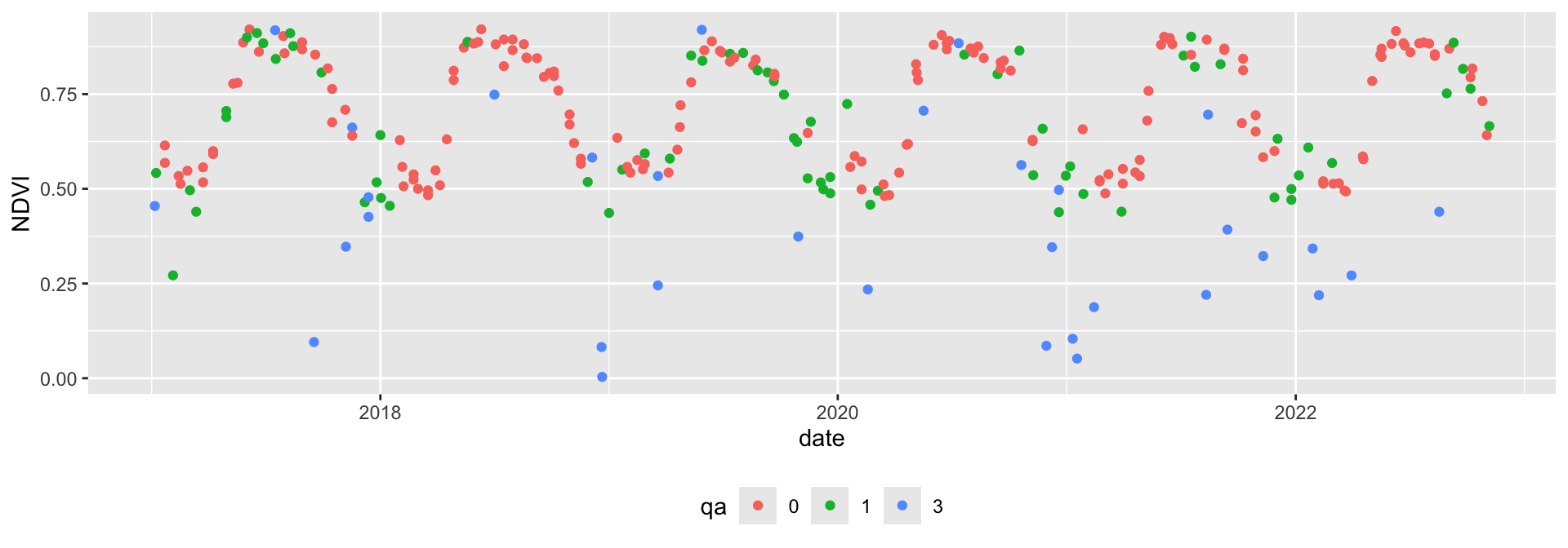
We can filter out cloudy and noise pixels based on the pixel reliability band.
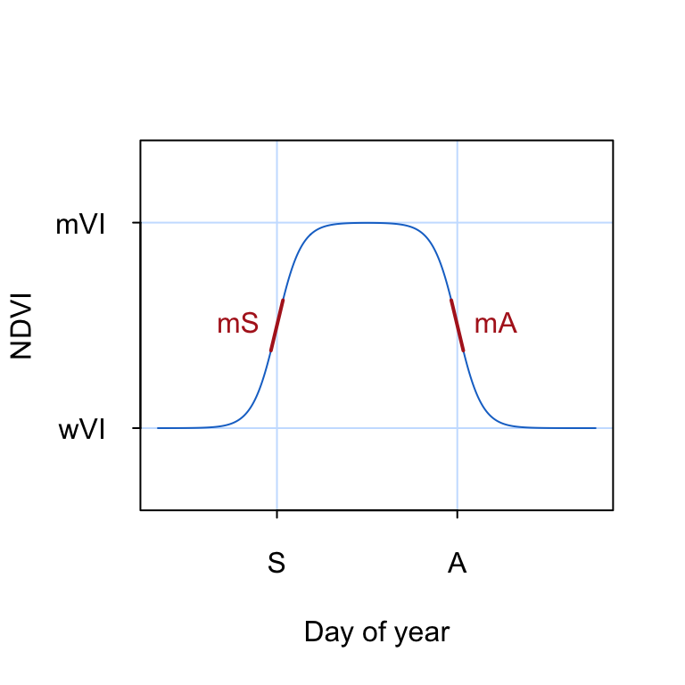
modis <- modis[modis$qa==0,]The double-logistic function is commonly used to describe the seasonal changes in NDVI associated with natural vegetation phenology (Figure 18.1). The double-logistic function is formulated after Beck et al. (2006) as follows:
\[\footnotesize g(t;mS,S,mA,A) = wVI + (mVI - wVI) \cdot (\frac{1}{1+e^{-mS*(t-S)}} + \frac{1}{1+e^{mA*(t-A)}} -1) \tag{18.2}\]
where \(t\) is time in day of year, \(wVI\) and \(mVI\) are the winter and maximum vegetation index, respectively, \(mS\) and \(mA\) are the green-up and senescence rate, respectively, and \(S\) and \(A\) are the start and end of season (day of year), respectively.
To visualize the double logisitic function, we convert Equation 18.2 into an R function dlFun() that takes a time argument t and a named vector of parameters p as input.
dlFun <- function(t, p){
  term1 <- (1 / (1 + exp(-p["mS"] * (t - p["S"]))))
  term2 <- (1 / (1 + exp( p["mA"] * (t - p["A"]))))
  return(p["wVI"] + (p["mVI"] - p["wVI"]) * (term1 + term2 - 1))
}
Now, let’s test the double logistic function by inserting some parameter values:
t <- 1:365 # Day of year
wVI <- 0.1 # Season minimum VI
mVI <- 0.6 # Season maximum VI
mS <- 0.1 # Green-up rate
mA <- 0.1 # Senescence rate
S <- 60 # Start of season
A <- 150 # End of season
start_params <- c(wVI=wVI, mVI=mVI, mS=mS, S=S, mA=mA, A=A)
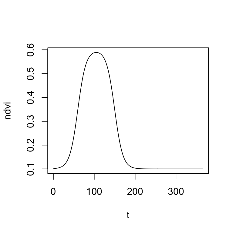
ndvi <- dlFun(t=t, start_params)
head(ndvi)[1] 0.1013658 0.1015090 0.1016672 0.1018419 0.1020348 0.1022479..and the corresponding plot of NDVI as a function of time \(t\):
Before we can fit the double-logistic function to our MODIS time series, it is important that we find some meaningful starting parameters. We can do this, by visually overlaying the MODIS NDVI time series of a single year with the double-logistic function. Then, manually change the parameters in the start_params vector (created above) and interactively adapt the double-logistic function to fit the MODIS data. The fit does not have to be perfect, but we want to start with a good first guess.
modis2021 <- modis[modis$year==2021,] # select data from year 2021
plot(ndvi ~ doy, data=modis2021, col=modis2021$qa, ylim=c(0,1)) # plot MODIS NDVI
lines(t, dlFun(t, start_params), col="blue") # add double-logistic function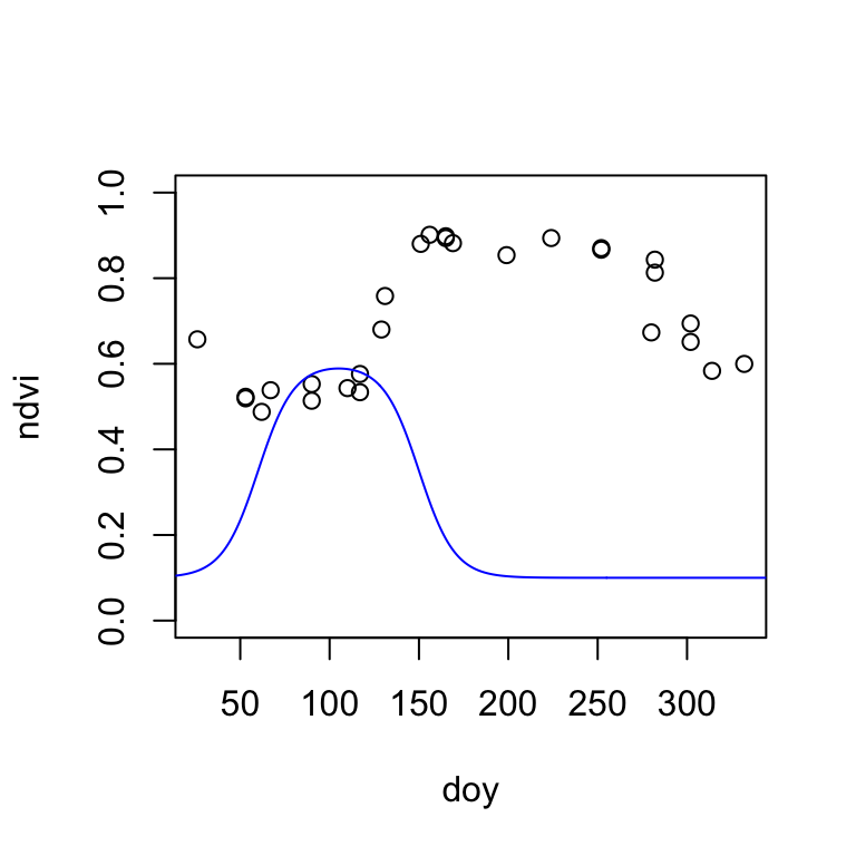
Once you visually estimated the starting parameters of the double-logistic function, it is time to fit the function to the MODIS data using non-linear least-squares regression. The nls() function (like lm()) takes a formula object. Because the equation of the double-logistic function is long (Equation 18.2), I write the formula in a separate line. We also must specify an na.action, in case of NA values in the data. Here, we omit all NA values.
start_params <- c(wVI=0.5, mVI=0.8, mS=0.1, S=100, mA=0.1, A=250)

formula <- ndvi ~ wVI + (mVI-wVI) * ((1 / (1 + exp(-mS * (doy - S)))) +  (1 / (1 + exp(mA * (doy -A)))) -1)

fit <- nls(formula, modis2021, start = start_params, na.action = "na.omit")
Let’s extract and inspect the function (phenological) parameters.
fitted_params <- coef(fit)
fitted_params
wVI mVI mS S mA A
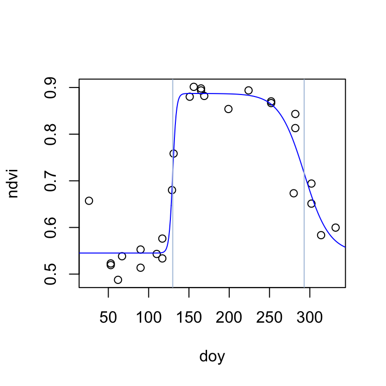
0.54515770 0.88725331 0.44829070 129.91357522 0.06402943 292.99196080 The start-of-season (inflection point) is estimated on day 130, and the end-of-season on day 293. The season NDVI minimum and maximum are estimated to be 0.55 and 0.89, respectively. Finnaly, the rate of change in NDVI is considerably higher during the start of season (0.45) than during the end-ofseason (0.06). Let’s visualize the fitted double-logistic function:
plot(ndvi ~ doy, data=modis2021)
lines(t, dlFun(t, fitted_params), col="blue")
abline(v=c(fitted_params["S"], fitted_params["A"]), col="lightsteelblue")