library(ggplot2)11 Quantitative accuracy
Packages
Background
Quantitative accuracy describes how close a model’s predicted values are to the actual observed values. It helps us understand how well a model performs in producing reliable numerical results. To measure quantitative accuracy (or prediction accuracy), we use statistical indicators such as Mean Absolute Error (MAE), Root Mean Squared Error (RMSE), and Bias. These measures allow us to compare models, identify systematic errors, and improve the overall quality of predictions.
The methods for estimating prediction error do not depend on the type of model being used for prediction. In the following, we will examine how accurately a simple linear regression model (see Section 10.6) can predict the observed values, but the same methods apply also to other types of regression models, i.e., models that have a continuous response.
vegdata <- read.csv('data/frac/NDVI_veg-ref.csv')
vegmod <- lm(vegcov ~ ndvi, data = vegdata)
summary(vegmod)
Call:
lm(formula = vegcov ~ ndvi, data = vegdata)

Residuals:
    Min      1Q  Median      3Q     Max
-15.146  -2.317   0.428   5.316  18.983

Coefficients:
            Estimate Std. Error t value Pr(>|t|)
(Intercept)   10.081      6.471   1.558    0.142
ndvi         108.514     10.226  10.611 4.46e-08 ***
---
Signif. codes:  0 '***' 0.001 '**' 0.01 '*' 0.05 '.' 0.1 ' ' 1

Residual standard error: 9.089 on 14 degrees of freedom
Multiple R-squared:  0.8894,    Adjusted R-squared:  0.8815
F-statistic: 112.6 on 1 and 14 DF,  p-value: 4.459e-08
The outputs of our regression model show the estimated model parameters (intercept and slope), their statistical significance, and the overall goodness of fit. In this case, NDVI explains 88.9% of the variance in vegetation cover. Although a good model fit often suggests strong predictive performance, this is not guaranteed. A model can appear to fit the observed data well while overfitting, capturing noise rather than the underlying relationship. To properly assess prediction accuracy and detect potential overfitting, additional methods are required.
Test data
Just as classification error is estimated on separate data, prediction error for continuous estimates is evaluated using an independent dataset, referred to here as vegtest.
vegtest <- read.csv('data/frac/NDVI_veg-testdata.csv')
head(vegtest)
vegcov ndvi
1 100 0.82
2 100 0.80
3 100 0.79
4 100 0.87
5 95 0.75
6 88 0.70We use the predict() function to apply the model (vegmod) to the test dataset vegtest. All we need is the model and a new data.frame. Important! The predict function matches the variables by name, so make sure the names are spelled correctly.
formula(vegmod)vegcov ~ ndviThe predict function uses the variable ndvi from vegtest to predict vegetation cover fractions. Let`s add these predictions as a new column to the test dataset.
vegtest$predicted <- predict(vegmod, vegtest)
head(vegtest)
vegcov ndvi predicted
1 100 0.82 99.06187
2 100 0.80 96.89160
3 100 0.79 95.80646
4 100 0.87 104.48756
5 95 0.75 91.46591
6 88 0.70 86.04023Scatter plot
Scatter plots are commonly used to assess quantitative accuracy by comparing observed and predicted values. Each point on the plot represents an observed (reference) value and its corresponding predicted value. In a way, the scatter plot for continuous data serves a similar role as a confusion matrix does for categorical predictions, such as land cover classes. To aid interpretation, a 1:1 line is added to the plot, which should not be confused with a regression line.
ggplot(vegtest, aes(x = vegcov, y = predicted)) +
  geom_point() +
  geom_abline(intercept = 0, slope = 1) +
  theme_classic()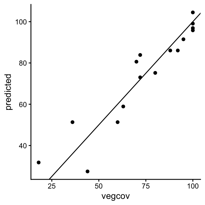
Intuitively, the observed and predicted vegetation cover fractions in our example appear to agree well. Most scatter points lie fairly close together, although the differences tend to be larger at low cover fractions and smaller at higher ones. But how can we quantify the degree of agreement or disagreement?
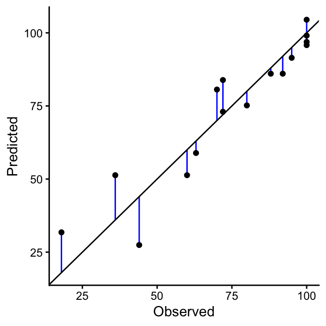
Prediction error
If the predicted and observed values were identical (i.e., showed 100% agreement), all points would lie exactly on the 1:1 line in the scatter plot (black line). Therefore, the degree of agreement can be assessed by measuring how far the individual points deviate from this line. Points that lie close to the 1:1 line indicate good agreement between predicted and observed values, while points farther away reflect larger prediction errors. Mathematically, this deviation is expressed as the difference between the predicted and observed values, \(\hat{y_i}\) - \(y_i\) (blue lines). Most quantitative measures of agreement are based on this difference, such as the Mean Absolute Error (MAE), Root Mean Squared Error (RMSE), and Bias.
RMSE and MSE
MAE (Mean Absolute Error) is the average of the absolute differences between predicted and observed values, treating all errors equally. RMSE (Root Mean Squared Error) is the square root of the average squared differences, giving greater weight to larger errors.
\(MAE = \frac{\sum_{i=1}^{n}|\hat{y_i}-y_i|}{n}\)
\(RMSE = \sqrt{\frac{\sum_{i=1}^{n}(\hat{y_i}-y_i)^2}{n}}\)
The RMSE is often higher than the MAE. It is more sensitive to outliers, but it can also be more appropriate for heteroscedastic errors, i.e., situations where the variability of the errors changes across the range of predicted values (e.g., biomass). In contrast, MAE treats all errors equally, providing a more balanced measure of overall prediction accuracy.
The RMSE and MAE are expressed in the same units as the predicted and observed values, which makes them intuitive to interpret. However, comparing errors in absolute terms can be challenging when the magnitude of the observed values varies widely or when comparing across different datasets or variables. In such cases, relative or normalized measures are often used to facilitate meaningful comparisons. For example, the relative RMSE is calculated by dividing the RMSE by the mean of the observed values, often expressed as a percentage:
\({RMSE\%} = 100 \times \frac{\text{RMSE}}{\bar{y}}\)
Bias
Bias measures the systematic error in predictions by quantifying the average difference between predicted (\(\hat{y_i}\)) and observed (\(y_i\)) values. It indicates whether a model tends to consistently overestimate or underestimate the true values. Note, bias is often defined as the difference between the mean predicted value and the mean observed value, which is mathematically equivalent to the average of the individual differences:
\(Bias = \bar{\hat{y}} - \bar{y} = \frac{1}{n} \sum_{i=1}^{n} (\hat{y_i} - y_i)\)
Note
Prediction error is the difference between the predicted value from a model (\(\hat{y_i}\)) and the actual observed value (\(y_i\)) for a given data point. It quantifies how far off a model’s prediction is from reality. Prediction errors can be summarized across all data points using metrics like MAE, RMSE, or Bias to evaluate overall model performance.
Regression
To check for systematic deviations from the 1:1 line, we can fit a line to the scatter plot. We do not do this to build a predictive model, but to describe the relationship between observed and predicted values. Ideally, the slope is close to 1 and the intercept is close to 0. Deviations from these values indicate biases, such as consistent over- or underprediction, or errors that depend on the value range.
ggplot(vegtest, aes(x = vegcov, y = predicted)) +
  geom_point() +
  geom_abline(intercept = 0, slope = 1) + # 1:1 line
  geom_smooth(method = "lm") + # regression line
  theme_classic()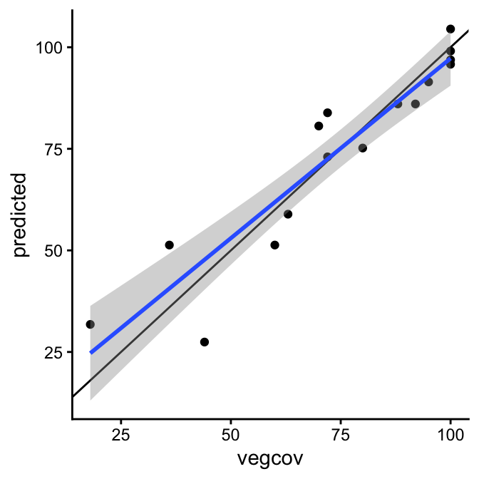
In our example, the simple linear regression line (blue line) shows a slight overprediction at low values and underprediction high values. This is also expressed in the regression coefficients.
yh_model <- lm(predicted ~ vegcov, data=vegtest)
coefficients(yh_model)
(Intercept) vegcov
8.7616705 0.8849317 The Pearson correlation coefficient (r) of the predicted versus observed values measures the strength and direction of the linear relationship between them. A value close to 1 indicates a strong positive linear relationship, meaning predictions closely follow the observed values, while a value near 0 indicates little or no linear association. This coefficient complements metrics like MAE or RMSE, which measure the size of errors, by showing the overall linear agreement between predictions and observations.
cor(vegtest$vegcov, vegtest$predicted)[1] 0.9366804