library(terra)
library(sf)7 Vector data
Packages
Background
In this chapter, you will learn how to read, create, and write vector data in R using the sf package. We will illustrate these skills with a practical example commonly used before a classification task. The example involves creating a spatial vector dataset (geopackage) from a text file containing point coordinates from a field survey (LUCAS, Section 14.2.2) and reprojecting the vector dataset to match the coordinate reference system of a Landsat satellite image.
sf package
The sf package provides classes to read, write, and manipulate vector data in R (Pebesma, 2022, 2018). The sf package supersedes the older sp package. Because the sp package has been around for a longer time, dependencies with some packages may still exist. But development of sp will eventually be stopped at some point. The letters sf stand for ‘simple features’ or ‘simple feature access’, which is a formal standard that will make handling and conversion of vector data easier.
The sf package represents simple features as native R objects, using simple data structures (S3 classes, lists, matrices, vectors). All functions and methods in sf that operate on spatial data are prefixed by st_, which refers to spatial and temporal. See also the package vignettes.
In the sf package three classes are used to represent simple features:
sf: a spatial data.frame with feature attributes and feature geometries. The geometry column is of classsfcand is typically called geometry or geom but any name can be used.sfc: the list-column with the geometries for each feature (record), which is composed ofsfg.sfg: the feature geometry of an individual simple feature, e.g. a point, linestring, multilinestring, polygon, multipolygon.
Read spatial vectors
read_sf and write_sf are aliases for st_read and st_write, respectively, with some modified default arguments.
sf_europe <- read_sf('data/landcov/cntry_boundary_europe-subset_epsg4326.gpkg')
sf_europe
Simple feature collection with 46 features and 6 fields (with 2 geometries empty)
Geometry type: MULTIPOLYGON
Dimension: XY
Bounding box: xmin: -10.47106 ymin: 34.92295 xmax: 40.21611 ymax: 71.12681
Geodetic CRS: WGS 84
# A tibble: 46 × 7
COUNTRY ISO_CC CONTINENT Land_Type Land_Rank COUNTRYAFF
<chr> <chr> <chr> <chr> <int> <chr>
1 Albania AL Europe Primary land 5 Albania
2 Andorra AD Europe Primary land 5 Andorra
3 Austria AT Europe Primary land 5 Austria
4 Belarus BY Europe Primary land 5 Belarus
5 Belgium BE Europe Primary land 5 Belgium
6 Bosnia and Herzegovina BA Europe Primary land 5 Bosnia and H…
7 Bulgaria BG Europe Primary land 5 Bulgaria
8 Croatia HR Europe Medium island 3 Croatia
9 Czech Republic CZ Europe Primary land 5 Czech Republ…
10 Denmark DK Europe Medium island 3 Denmark
# ℹ 36 more rows
# ℹ 1 more variable: geom <MULTIPOLYGON [°]>Create spatial vectors
The LUCAS samples (Section 14.2.2) are recorded in a text file, which contains the plot id, the land cover class, and longitude (X_WGS84) and latitude (Y_WGS84). We are going to use only a small subset of the LUCAS 2015 sample collected over the Berlin-Brandenburg region.
lucas_df <- read.csv('data/landcov/landcover_lucas2015_bbrdbg_ascii.csv')
head(lucas_df)
POINT_ID class X_WGS84 Y_WGS84
1 45683256 1 13.62719 52.35809
2 44943412 1 12.62505 53.78711
3 45223262 1 12.95604 52.43064
4 45383392 1 13.27803 53.59146
5 45783412 1 13.89771 53.75314
6 44863358 1 12.47545 53.30473To convert the data.frame into spatial data.frame (sf object), we can use the st_as_sf() function.
lucas_sf <- st_as_sf(lucas_df, coords=c('X_WGS84','Y_WGS84'), remove=F)
lucas_sf
Simple feature collection with 4472 features and 4 fields
Geometry type: POINT
Dimension: XY
Bounding box: xmin: 11.61411 ymin: 51.91658 xmax: 15.40705 ymax: 54.32519
CRS: NA
First 10 features:
POINT_ID class X_WGS84 Y_WGS84 geometry
1 45683256 1 13.62719 52.35809 POINT (13.62719 52.35809)
2 44943412 1 12.62505 53.78711 POINT (12.62505 53.78711)
3 45223262 1 12.95604 52.43064 POINT (12.95604 52.43064)
4 45383392 1 13.27803 53.59146 POINT (13.27803 53.59146)
5 45783412 1 13.89771 53.75314 POINT (13.89771 53.75314)
6 44863358 1 12.47545 53.30473 POINT (12.47545 53.30473)
7 45863296 1 13.92287 52.70861 POINT (13.92287 52.70861)
8 44323244 1 11.62707 52.29442 POINT (11.62707 52.29442)
9 44383354 1 11.75417 53.28137 POINT (11.75417 53.28137)
10 44883342 1 12.49709 53.16044 POINT (12.49709 53.16044)Coordinate system
So far so good, but our newly created spatial vector data frame is missing a coordinate reference system. Our LUCAS sample coordinates are in a geographic coordinate system with WGS-84 as spheroid and datum (EPSG=4326). There are different format conventions for projections. A common format is the proj4 string, which we can grab from this website. Fortunately, also sf can also read EPSG codes, which makes the process easy:
# either as proj4 string
proj <- "+proj=longlat +ellps=WGS84 +datum=WGS84 +no_defs"

# or EPSG code
proj <- 4326
We can now add the coordinate reference system when creating the spatial vectors.
lucas_sf <- st_as_sf(lucas_df, coords=c('X_WGS84','Y_WGS84'), remove=F, crs=proj)
lucas_sf
Simple feature collection with 4472 features and 4 fields
Geometry type: POINT
Dimension: XY
Bounding box: xmin: 11.61411 ymin: 51.91658 xmax: 15.40705 ymax: 54.32519
Geodetic CRS: WGS 84
First 10 features:
POINT_ID class X_WGS84 Y_WGS84 geometry
1 45683256 1 13.62719 52.35809 POINT (13.62719 52.35809)
2 44943412 1 12.62505 53.78711 POINT (12.62505 53.78711)
3 45223262 1 12.95604 52.43064 POINT (12.95604 52.43064)
4 45383392 1 13.27803 53.59146 POINT (13.27803 53.59146)
5 45783412 1 13.89771 53.75314 POINT (13.89771 53.75314)
6 44863358 1 12.47545 53.30473 POINT (12.47545 53.30473)
7 45863296 1 13.92287 52.70861 POINT (13.92287 52.70861)
8 44323244 1 11.62707 52.29442 POINT (11.62707 52.29442)
9 44383354 1 11.75417 53.28137 POINT (11.75417 53.28137)
10 44883342 1 12.49709 53.16044 POINT (12.49709 53.16044)With the function st_crs(), we can extract the coordinate reference system.
st_crs(lucas_sf)Coordinate Reference System:
User input: EPSG:4326
wkt:
GEOGCRS["WGS 84",
ENSEMBLE["World Geodetic System 1984 ensemble",
MEMBER["World Geodetic System 1984 (Transit)"],
MEMBER["World Geodetic System 1984 (G730)"],
MEMBER["World Geodetic System 1984 (G873)"],
MEMBER["World Geodetic System 1984 (G1150)"],
MEMBER["World Geodetic System 1984 (G1674)"],
MEMBER["World Geodetic System 1984 (G1762)"],
MEMBER["World Geodetic System 1984 (G2139)"],
MEMBER["World Geodetic System 1984 (G2296)"],
ELLIPSOID["WGS 84",6378137,298.257223563,
LENGTHUNIT["metre",1]],
ENSEMBLEACCURACY[2.0]],
PRIMEM["Greenwich",0,
ANGLEUNIT["degree",0.0174532925199433]],
CS[ellipsoidal,2],
AXIS["geodetic latitude (Lat)",north,
ORDER[1],
ANGLEUNIT["degree",0.0174532925199433]],
AXIS["geodetic longitude (Lon)",east,
ORDER[2],
ANGLEUNIT["degree",0.0174532925199433]],
USAGE[
SCOPE["Horizontal component of 3D system."],
AREA["World."],
BBOX[-90,-180,90,180]],
ID["EPSG",4326]]With the function st_crs(), we can also redefine the coordinate reference system.
st_crs(lucas_sf) <- 4326Plot spatial vectors
The basic plot() function works with sf objects. If you use plot() directly on the spatial vector all feature attributes are plotted. For more information see here.
plot(sf_europe, max.plot=3)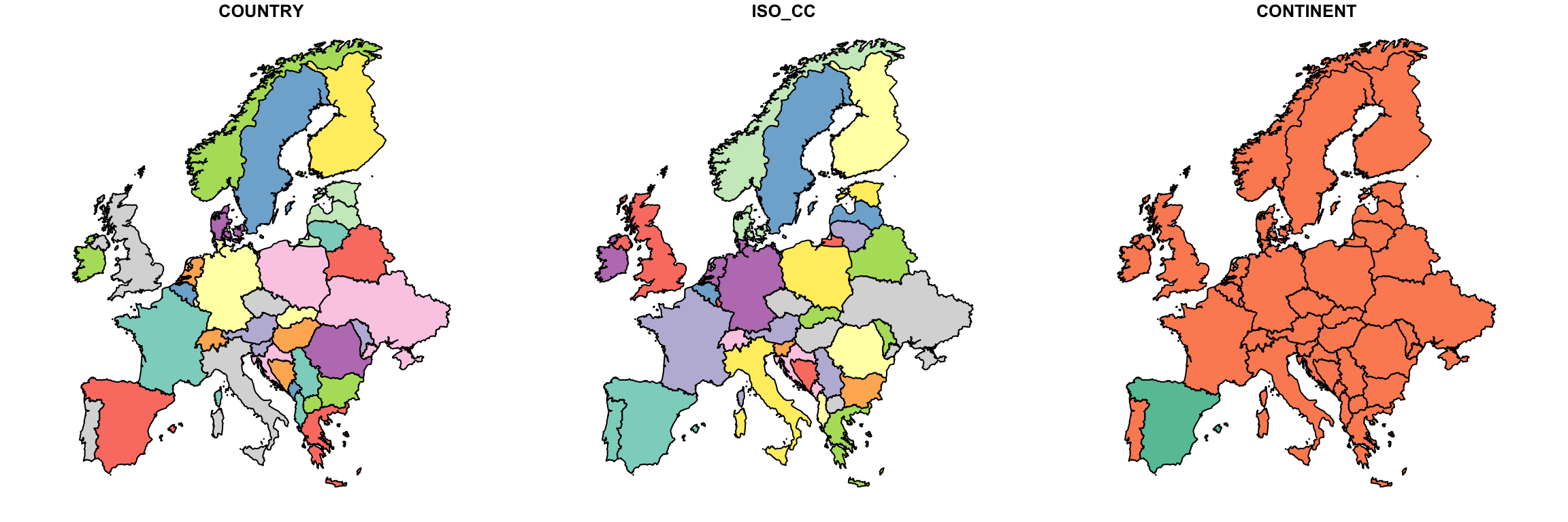
We can also plot a single attribute,
plot(sf_europe["ISO_CC"])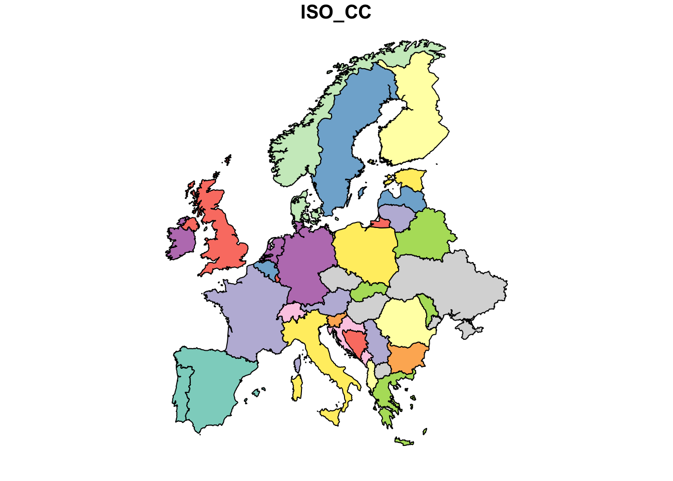
or only the geometry. Here, we also add the geometry of the LUCAS points.
plot(st_geometry(sf_europe), xlim=c(10, 15), ylim=c(51, 55))
plot(st_geometry(lucas_sf), add=T, cex=0.1, col=2)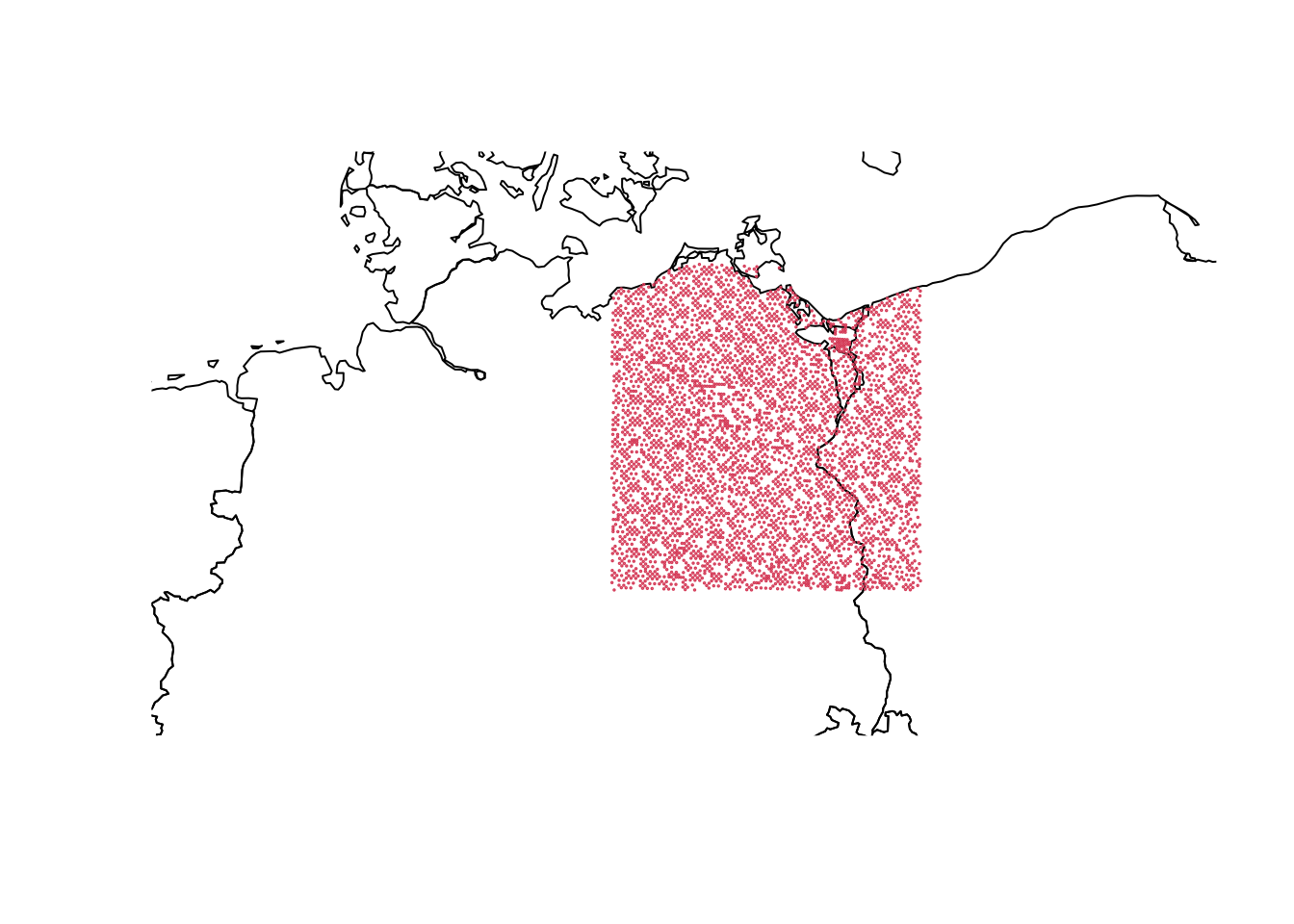
Reproject
With st_stransform(), we can reproject the spatial vectors to another coordinate reference system, e.g. EPSG=3035.
lucas_3035 <- st_transform(lucas_sf, st_crs(3035))Alternatively, we can automatically reproject the LUCAS data to match another dataset. For example, if we want to overlay the vector data with a Landsat image, we need to project (st_transform()) the LUCAS samples into the coordinate system of the Landsat image. The example below involves reading the Landsat image and extracting its coordinate reference system. You’ll notice, the Landsat image comes in UTM 33N.
l8tc <- rast('data/landcov/LC08_L2SP_193023_20170602_20200903_02_T1_tc.tif')
names(l8tc) <- c("tcb", "tcg", "tcw")

l8img_proj <- terra::crs(l8tc, proj=T)
l8img_proj
[1] "+proj=utm +zone=33 +datum=WGS84 +units=m +no_defs"lucas_utm <- st_transform(lucas_sf, l8img_proj)
lucas_utmSimple feature collection with 4472 features and 4 fields
Geometry type: POINT
Dimension: XY
Bounding box: xmin: 267524.2 ymin: 5751910 xmax: 527870.9 ymax: 6022165
Projected CRS: +proj=utm +zone=33 +datum=WGS84 +units=m +no_defs
First 10 features:
POINT_ID class X_WGS84 Y_WGS84 geometry
1 45683256 1 13.62719 52.35809 POINT (406511.9 5801754)
2 44943412 1 12.62505 53.78711 POINT (343543.4 5962453)
3 45223262 1 12.95604 52.43064 POINT (361039 5810902)
4 45383392 1 13.27803 53.59146 POINT (386028.4 5939447)
5 45783412 1 13.89771 53.75314 POINT (427319.9 5956620)
6 44863358 1 12.47545 53.30473 POINT (331787.3 5909142)
7 45863296 1 13.92287 52.70861 POINT (427228.8 5840401)
8 44323244 1 11.62707 52.29442 POINT (270002.1 5799144)
9 44383354 1 11.75417 53.28137 POINT (283622.9 5908486)
10 44883342 1 12.49709 53.16044 POINT (332667 5893044)Write spatial vectors
Write spatial data.frame to file as geopackage. The output format is automatically recognized based on the file ending.
write_sf(lucas_utm, "data/landcov/landcover_lucas2015_bbrdbg.gpkg")Plot on RGB image
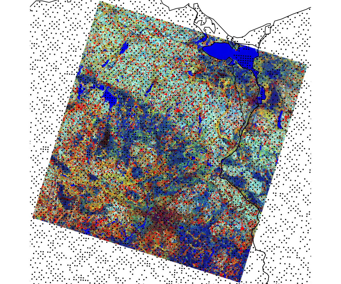
plotRGB(l8tc, r = 1, g= 2, b = 3, stretch = "hist")
plot(st_geometry(st_transform(sf_europe, crs=l8img_proj)), add=T)
plot(st_geometry(lucas_utm), add = TRUE, cex=0.3, pch=16)