library(prosail)
library(ggplot2)
library(tidyr)
library(dplyr)9 Field spectra
Packages
ASD FieldSpec
In this exercise, we will analyze data collected by an ASD FieldSpec 3 field spectrometer. The ASD FieldSpec 3 spectroradiometer has a spectral range of 350–2500 nm and measures solar reflectance, radiance, and irradiance. Key specifications include a spectral resolution of 3 nm at 700 nm and 10 nm at 1400/2100 nm, and a sampling interval of 1.4 nm (350-1000 nm) and 2.0 nm (1000-2500 nm).
Example data
The ASD FieldSpec 3 was used to take the following measurements: The white reference and target surfaces were positioned between the sun and the observer, forming a triangle with the sun, target, and sensor within the so-called solar principal plane. The instrument head was held at a constant height and oriented in the nadir direction.
Three different target measurements were conducted on the lawn in front of the institute, each preceded and followed by white reference measurements: a) white reference, b) target 1: nadir within the solar principal plane, c) target 2: 30° to the left of the solar principal plane, d) target 3: 30° to the right of the solar principal plane, e) white reference.
Each target and white reference measurement was repeated five times, resulting in a total of 25 measurements. The data was exported to the file vegetation.txt. Below, you see the first few lines of the data.frame, if you read in the file correctly (exercise). The first column represents wavelength in \(nm\), the remaining 25 columns represent the spectral radiance measurements (\(W * m^{-2} * sr^{-1} * nm^{-1}\)).
head(asd_rad) V1 V2 V3 V4 V5 V6 V7 V8 V9 V10 V11
1 350 0.110569 0.110474 0.110599 0.110658 0.110505 0.001638 0.001640 0.001610 0.001607 0.001635
2 351 0.111600 0.111487 0.111629 0.111665 0.111516 0.001649 0.001672 0.001643 0.001619 0.001625
3 352 0.113454 0.113337 0.113498 0.113527 0.113381 0.001693 0.001707 0.001678 0.001664 0.001664
4 353 0.115070 0.114949 0.115121 0.115150 0.114994 0.001734 0.001740 0.001705 0.001705 0.001699
5 354 0.115721 0.115582 0.115751 0.115779 0.115586 0.001744 0.001770 0.001715 0.001715 0.001689
6 355 0.116074 0.115935 0.116119 0.116147 0.115953 0.001739 0.001767 0.001693 0.001711 0.001701
V12 V13 V14 V15 V16 V17 V18 V19 V20 V21
1 0.001512 0.001543 0.001484 0.001517 0.001484 0.001512 0.001512 0.001512 0.001453 0.001453
2 0.001506 0.001536 0.001500 0.001553 0.001500 0.001506 0.001506 0.001506 0.001470 0.001470
3 0.001547 0.001576 0.001532 0.001591 0.001532 0.001532 0.001532 0.001517 0.001518 0.001503
4 0.001590 0.001613 0.001562 0.001613 0.001568 0.001562 0.001562 0.001533 0.001562 0.001527
5 0.001603 0.001605 0.001574 0.001605 0.001601 0.001574 0.001574 0.001546 0.001574 0.001520
6 0.001600 0.001618 0.001590 0.001582 0.001600 0.001590 0.001572 0.001545 0.001555 0.001517
V22 V23 V24 V25 V26
1 0.113098 0.113744 0.114670 0.113219 0.112760
2 0.114112 0.114737 0.115654 0.114207 0.113784
3 0.115993 0.116620 0.117554 0.116080 0.115657
4 0.117629 0.118261 0.119226 0.117722 0.117285
5 0.118255 0.118875 0.119884 0.118366 0.117917
6 0.118572 0.119219 0.120200 0.118719 0.118275
Tip
We repeated each measurement five times to reduce noise from slight illumination changes or hand movements. In your assignment, you will average each repeated measurement to yield a single measurement for the white reference and each target measurement, respectively. See Section 5.3.2 on how to apply functions over entire array margins (rows or columns). You will also convert for each target the spectral radiance in reflectance measurements.
Reflectance data
The reflectance measurements of the three targets are also available in the following csv file. You can read them into a data.frame using the read.csv function.
asd <- read.csv("data/spec/vegetation_spectra.csv")
head(asd)
wavelength target1 target2 target3
1 350 0.01451402 0.01346073 0.01328577
2 351 0.01452241 0.01343783 0.01319543
3 352 0.01463057 0.01353754 0.01323121
4 353 0.01472962 0.01363644 0.01329321
5 354 0.01473565 0.01363470 0.01329332
6 355 0.01465436 0.01359754 0.01323845To plot all three targets with ggplot, we first need to reshape the data frame from wide to long format. In the wide format, measurements for each target are stored in separate columns, repeating similar information. Converting the data to long format removes this redundancy by creating two new variables: one column for the measurement value (reflectance) and another identifying the target type (target). This structure is easier for ggplot to work with, especially when plotting multiple groups. We can perform this transformation using tidyr::pivot_longer() (Section 4.3).
asd_all <- tidyr::pivot_longer(asd, cols = starts_with("target"),
                               names_to = "target",
                               values_to = "reflectance")
asd_all
# A tibble: 6,453 × 3
wavelength target reflectance
<int> <chr> <dbl>
1 350 target1 0.0145
2 350 target2 0.0135
3 350 target3 0.0133
4 351 target1 0.0145
5 351 target2 0.0134
6 351 target3 0.0132
7 352 target1 0.0146
8 352 target2 0.0135
9 352 target3 0.0132
10 353 target1 0.0147
# ℹ 6,443 more rowsNow we can plot reflectance against wavelength for each target, allowing us to compare and visually interpret the three spectral signatures.
ggplot(asd_all, aes(x = wavelength, y = reflectance, color = target)) +
  geom_line() +
  labs(x = "Wavelength (nm)", y = "Reflectance", color = "Target") +
  theme_classic()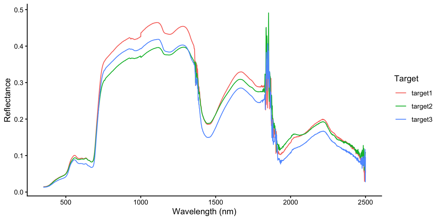
Hyperspectral indices
Spectral indices are transformations of few selected spectral bands to capture or enhance certain physical gradients such as vegetation structure and greenness, and biochemical gradients related to plant constituents, canopy moisture, and nutrient content. Spectral indices usually capture distinct absorption features, many of which are visible in multi-spectral data but some are only (or better) detectable with hyperspectral data (Roberts et al., 2018). See Roberts et al. (2018) for a more complete overview of hyperspectral indices.
Cellulose Absorption Index
The Cellulose Absorption Index (CAI) detects a narrow absorption feature in the short-wave infrared region, which is correlated with the amount of non-photosynthetic active radiation (Daughtry, 2001).
\(CAI = 0.5 * (\rho_{2.0} + \rho_{2.2}) - \rho_{2.1}\)
where \(\rho_{2.0}\), \(\rho_{2.2}\), and \(\rho_{2.1}\) are the reflectance factors at respective wavelengths in \(\mu m\).
The example below, calculates the CAI for all three ASD targets at ones. Note, the -1 removes the first (wavelength) column, and our wavelengths are in nm.
r2019 <- asd[asd$wavelength == 2019, -1]
r2019
target1 target2 target3
1670 0.1473424 0.1584428 0.1172318r2206 <- asd[asd$wavelength == 2206, -1]
r2206 target1 target2 target3
1857 0.1979317 0.1912445 0.1656753r2109 <- asd[asd$wavelength == 2109, -1]
r2109 target1 target2 target3
1760 0.1654468 0.1634123 0.1388659cai <- 0.5 * (r2019 + r2206) - r2109
cai target1 target2 target3
1670 0.007190203 0.01143138 0.002587692Photochemical Reflectance Index
The Photochemical Reflectance Index (PRI) is a measure used to assess photosynthetic light-use efficiency in plants (Gamon et al., 1997). It is sensitive to changes in carotenoid pigments, particularly xanthophylls, which are involved in the plant’s response to light and stress. The PRI is calculated using reflectance measurements at specific wavelengths (typically 531 nm and 570 nm) and is used to monitor vegetation health and productivity.
\(PRI = \frac{\rho_{531} - \rho_{570}}{\rho_{531} + \rho_{570}}\)
r531 <- asd[asd$wavelength == 531, -1]
r570 <- asd[asd$wavelength == 570, -1]
pri <- (r531 - r570) / (r531 + r570)
pri
target1 target2 target3
182 -0.0627118 -0.07480126 -0.06208184Spectral resampling
Spectral resampling is the process of adjusting hyperspectral (continuous) or high-resolution spectral data to match the spectral characteristics of another sensor with broader wavelengths, e.g., multi-spectral satellite sensors such as Landsat’s OLI and Sentinel-2 MSI. A simple approach is the boxcar method, which assumes uniform sensitivity across each band, while a more accurate approach applies the spectral response functions (SRFs) of the target sensor to weight the data according to the sensor’s true wavelength-dependent sensitivity. This ensures a more realistic simulation of how the target sensor would capture the same scene.
Box-car method
The box-car method simply averages the hyperspectral reflectance factors within each band, defined by its full width at half maximum (FWHM). This approach assumes that each band exhibits a flat, uniform sensitivity across its bandwidth and zero sensitivity outside it. Consequently, each band is represented as a rectangular “box” filter centered at a given wavelength. While the method is straightforward and does not require detailed sensor response data, its oversimplified nature can introduce errors, particularly for sensors with wide bands or for spectra that contain sharp absorption or reflectance features.
Spectral Response Function (SRF)
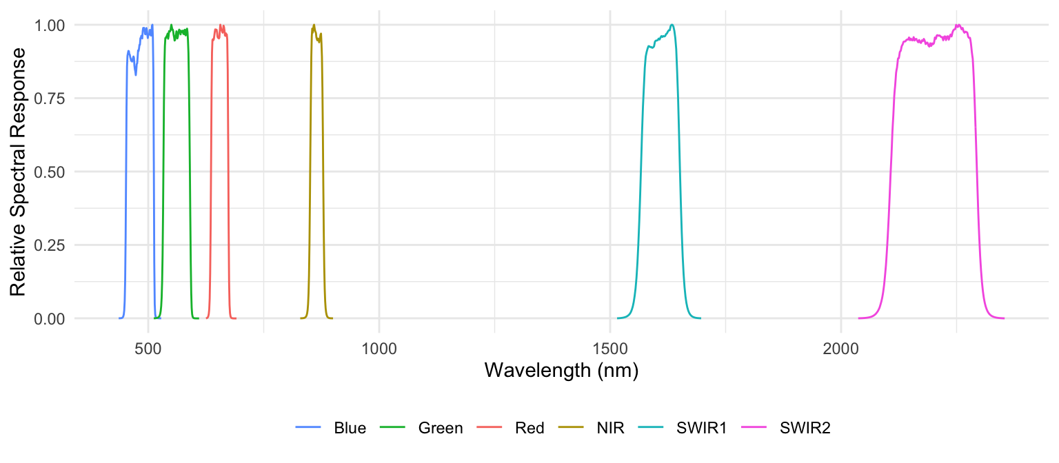
The spectral response function (SRF) resampling method applies the actual wavelength-dependent sensitivity of each target sensor band when integrating hyperspectral data. Instead of assuming uniform response, this approach weights the hyperspectral reflectance values by the sensor’s SRF before averaging. Each band’s SRF characterizes how the sensor responds across its spectral range (Figure 9.1). The resampled reflectance for a band is therefore computed as the weighted mean of the hyperspectral spectrum, normalized by the integrated SRF. Although this method requires access to detailed sensor response data and involves slightly higher computational effort, it provides a far more accurate and physically realistic simulation of the target sensor’s spectral measurements.
We can conduct spectral response function resampling using the prosail package. The package includes SRF’s for different sensors including Sentinel-2 MSI and Landsat ETM+ and OLI. The SRF is stored in R objects of type list and named as follows: Landsat_7, Landsat_8, and Sentinel_2. The code below shows that the Landsat_7 object contains several slots including the spectral band names (Spectral_Bands) and wavelength (Central_WL). We need this information later, because we want to exclude the atmospheric bands and the pan band from Landsat 7 and Landsat 8 from further analysis.
str(Landsat_8)List of 4
$ Spectral_Response: num [1:9, 1:2101] 0 0 0 0 0 0 0 0 0 0 ...
..- attr(*, "dimnames")=List of 2
.. ..$ : chr [1:9] "CoastalAerosol" "Blue" "Green" "Red" ...
.. ..$ : NULL
$ Spectral_Bands : chr [1:9] "CoastalAerosol" "Blue" "Green" "Red" ...
$ Original_Bands : int [1:2101] 400 401 402 403 404 405 406 407 408 409 ...
$ Central_WL : num [1:9] 443 482 562 655 865 ...Landsat_8$Spectral_Bands[1] "CoastalAerosol" "Blue" "Green" "Red" "NIR"
[6] "Cirrus" "SWIR1" "SWIR2" "Pan" Landsat_8$Central_WL[1] 443.0 482.5 562.5 655.0 865.0 1375.0 1610.0 2200.0 590.0Landsat-7 ETM+
Let’s simulate Landsat-7 ETM+ reflectance from ASD target 1:
l7sim <- applySensorCharacteristics(wvl = asd$wavelength,
                                    SRF = Landsat_7,
                                    InRefl = asd$target1)

# add wavelengths
l7sim$wavelength <- Landsat_7$Central_WL

# add band names
l7sim$names <- Landsat_7$Spectral_Bands

# rename to target 1
names(l7sim)[1]  <- "target1"

# remove PAN band
l7sim <- l7sim[l7sim$names != "PAN", ]
l7sim
target1 wavelength names
1 0.04575657 477.5 Blue
2 0.09231021 560.0 Green
3 0.08897050 661.5 Red
4 0.39403979 835.0 NIR
5 0.30761887 1648.0 SWIR1
6 0.17187565 2204.5 SWIR2Landsat-8 OLI
Now, let’s resample the spectra from target 1 to Landsat-8 OLI reflectance:
l8sim <- applySensorCharacteristics(wvl = asd$wavelength,
                                           SRF = Landsat_8,
                                           InRefl = asd$target1)

# add wavelengths
l8sim$wavelength <- Landsat_8$Central_WL

# add band names
l8sim$names <- Landsat_8$Spectral_Bands

# rename to target 1
names(l8sim)[1] <- "target1"

# remove PAN band Coastal Aerosol band
l8sim <- l8sim[!l8sim$names %in% c("Pan", "CoastalAerosol"), ]
l8sim
target1 wavelength names
2 0.04646105 482.5 Blue
3 0.09547598 562.5 Green
4 0.08687663 655.0 Red
5 0.40696817 865.0 NIR
6 0.33091947 1375.0 Cirrus
7 0.30363524 1610.0 SWIR1
8 0.18197912 2200.0 SWIR2Sentinel-2
Now, let’s resample the spectra from target 1 to Sentinel-2 MSI reflectance:
s2sim <- applySensorCharacteristics(wvl = asd$wavelength,
                                           SRF = Sentinel_2,
                                           InRefl = asd$target1)

# add wavelengths
s2sim$wavelength <- Sentinel_2$Central_WL

# add band names
s2sim$names <- Sentinel_2$Spectral_Bands

# rename to target 1
names(s2sim)[1]  <- "target1"

s2sim
target1 wavelength names
1 0.05150729 492.7 B2
2 0.09790946 559.8 B3
3 0.08464024 664.6 B4
4 0.17638896 704.1 B5
5 0.33510762 740.5 B6
6 0.37181544 782.8 B7
7 0.39348691 832.8 B8
8 0.40702736 864.7 B8A
9 0.30640136 1613.7 B11
10 0.18382539 2202.4 B12Compare sensors
To compare the original ASD hyperspectral measurements with the resampled multispectral data, we first add a sensor column to each dataset to identify its source. We then combine all datasets using dplyr’s bind_rows() into a single data.frame, keeping only the columns needed for plotting: wavelength, reflectance (target1), and sensor name.
# add sensor to each dataset
l7sim$sensor <- "Landsat-7"
l8sim$sensor <- "Landsat-8"
s2sim$sensor <- "Sentinel-2"
asd$sensor <- "ASD"

# stack all datasets
spec_all <- dplyr::bind_rows(asd, l7sim, l8sim, s2sim)
Note
The function bind_rows() from dplyr is more flexible than rbind() from base R: it automatically handles missing columns by filling them with NA values, and it works more efficiently with lists of data frames. In contrast, rbind() requires all data frames to have identical column names and types.
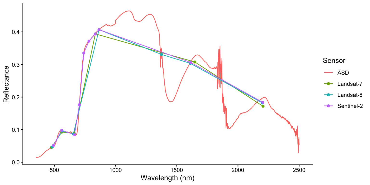
This combined data.frame allows us to create a single ggplot that displays all spectra with automatic color-coding by sensor. We draw continuous lines for all sensors and overlay points only for the multispectral sensors (Landsat-7, Landsat-8, and Sentinel-2) to highlight their discrete band positions, making it easy to see how the coarser spectral resolution of satellite sensors compares to the continuous ASD measurements.
ggplot(spec_all, aes(x = wavelength, y = target1, color = sensor)) +
  geom_line() +
  geom_point(data=spec_all[spec_all$sensor != "ASD", ]) +
  labs(x = "Wavelength (nm)", y = "Reflectance", color = "Sensor") +
  theme_classic()