library(terra)
library(sf)
library(randomForest)
library(ggplot2)14 Classification
Packages
Background
The objective of this exercise is to create a land cover map using Landsat data (as predictors) and LUCAS data (as reference).
Landsat
We will use a relatively cloud-free Landsat-8 image acquired on June 2, 2017 over Berlin (Path 193, Row 23). The image has already been transformed into the tasseled-cap components—brightness (TCB), greenness (TCG), and wetness (TCW) (see Section 12.5).
l8tc <- rast('data/landcov/LC08_L2SP_193023_20170602_20200903_02_T1_tc.tif')
names(l8tc) <- c("tcb", "tcg", "tcw")
LUCAS
The LUCAS (Land Use/Cover Area frame Survey) survey is a field-based monitoring program conducted by Eurostat that collects harmonized data on land use and land cover across the European Union. It involves in-situ observations at approximately 350,000 locations, recording information on agriculture, soil, and other environmental characteristics. The data support environmental monitoring (e.g., soil quality, degradation, and biodiversity), provide evidence for EU agricultural and environmental policy, and serve as a technical resource for calibrating satellite imagery and maintaining reference points for specialized studies.
Here we are going to use only a small subset of the LUCAS 2015 sample collected over the Berlin-Brandenburg region.
lucas_utm <- st_read("data/landcov/landcover_lucas2015_bbrdbg.gpkg", quiet = TRUE)
Tip
If you have not already done so, review Chapter 7 to learn about the sf package and the steps for creating the geopackage used above.
Look-up table
Before building a classification model, it is good practice to create a look-up table (LUT) that stores the class codes and corresponding class names. This approach prevents you from hard-coding class information directly in your script and keeps your workflow more organized, reproducible, and adaptable to changes.
By storing this information in an external file, you effectively create a piece of metadata for your classification outputs. The LUT can also include additional attributes that are useful later in the analysis, such as color codes for visualization, class descriptions, or hierarchical groupings (e.g., forest vs. non-forest).
The code below reads our LUT for a simplified version of the LUCAS land cover classification. The LUT also stores colors as RGB values. To use these colors in R plots, we need to convert the RGB values to HEX color codes and add them to the LUT as a new column.
lut <- read.csv('data/landcov/landcover_lucas2015_legend.csv')
lut$color <- rgb(lut$R, lut$G, lut$B)
lut
class label R G B color
1 1 artificial 1.00 0.00 0.00 #FF0000
2 2 cropland 1.00 1.00 0.00 #FFFF00
3 3 broadleaf 0.00 0.78 0.00 #00C700
4 4 conifer 0.00 0.39 0.39 #006363
5 5 shrub 1.00 0.39 0.00 #FF6300
6 6 grass 0.78 0.78 0.39 #C7C763
7 7 water 0.00 0.00 1.00 #0000FFTraining data
Extract pixel values
The extract() function is a versatile function in the terra package that allows you to retrieve raster values corresponding to the locations of spatial vector data, such as points, lines, or polygons. When using points, a single raster value per pixel is returned. When using lines or polygons, multiple raster values may fall within each feature. In this case, you can provide a summary function (e.g., mean, sum, min, max) via the fun argument to aggregate the raster values over the feature. Setting na.rm = TRUE ensures that missing values are ignored during the aggregation.
To create a training dataset, we extract the tasseled cap values for each LUCAS location. Since extract() returns NA when a spatial feature (point, line, or polygon) overlaps only missing raster values, these entries must be removed from the training data. A training dataset cannot contain missing values, so filtering out these NAs is essential.
train_df <- terra::extract(l8tc, lucas_utm, bind = TRUE)
train_df <- na.omit(as.data.frame(train_df))
head(train_df, 3)
POINT_ID class X_WGS84 Y_WGS84 tcb tcg tcw
1 45683256 1 13.62719 52.35809 0.3300084 0.1702113 -0.1117129
2 44943412 1 12.62505 53.78711 0.3739685 0.2057397 -0.1467545
3 45223262 1 12.95604 52.43064 0.3440875 0.1344330 -0.1395941To include the attributes of the spatial vector along with the extracted raster values, set bind = TRUE. In this case, a SpatVector (terra’s vector object) is returned, which can then be coerced back into a data.frame. If bind is not set, extract() returns a data.frame of raster values only. You can then use cbind() to combine it with the attributes of the spatial vector manually.
Prepare response variable
The LUCAS class labels are stored as numeric values. To build a classification model, we need to convert these numeric codes into a categorical variable. Create a new column landcover in the train_df data frame that stores the land-cover class as a factor (Section 2.2), using the class names from the look-up table as labels.
Explore training data
We have now assembled a training dataset that contains the response variable (landcover) and the predictor variables (tasseled cap). Before we dive into the classification, it is a good idea to explore the training dataset regarding the distribution of samples per land cover class and the correlation between land cover and our response variables.
Using the table() function, we can summarize the number of observations per land cover class:
table(train_df$landcover)
artificial   cropland  broadleaf    conifer      shrub      grass      water
       147       1003        293        458         28        486        171
To get a first idea, how and if the tasseled cap values differ by land cover, we can use boxplot(). How distinct are the land cover classes spectrally?
boxplot(tcw ~ landcover, data=train_df)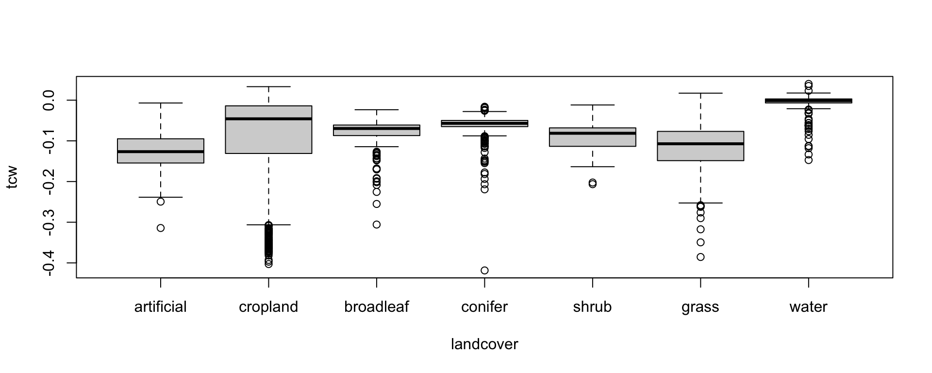
Boxplots allow us to visualize only one tasseled-cap component at a time. To explore relationships between two components simultaneously, we can use scatterplots. Here, we will use the ggplot2 package because it offers greater flexibility. For example, to differentiate land-cover classes in the scatterplot, we can assign the landcover column of our data.frame to the color option (aes(..., color = landcover)). We can also manually specify the colors associated with each class based on the colors from our LUT.
Let’s, plot tasseled-cap greenness against brightness, using the LUT colors to visualize the land-cover classes.
ggplot(train_df, aes(x = tcb, y = tcg, color = landcover)) +
  geom_point(alpha = 0.4) +
  scale_color_manual(values = setNames(lut$color, lut$label)) +
  labs(x = "Brightness",
       y = "Greenness",
       color = "Land Cover") +
  theme_classic() +
  theme(legend.position = "right")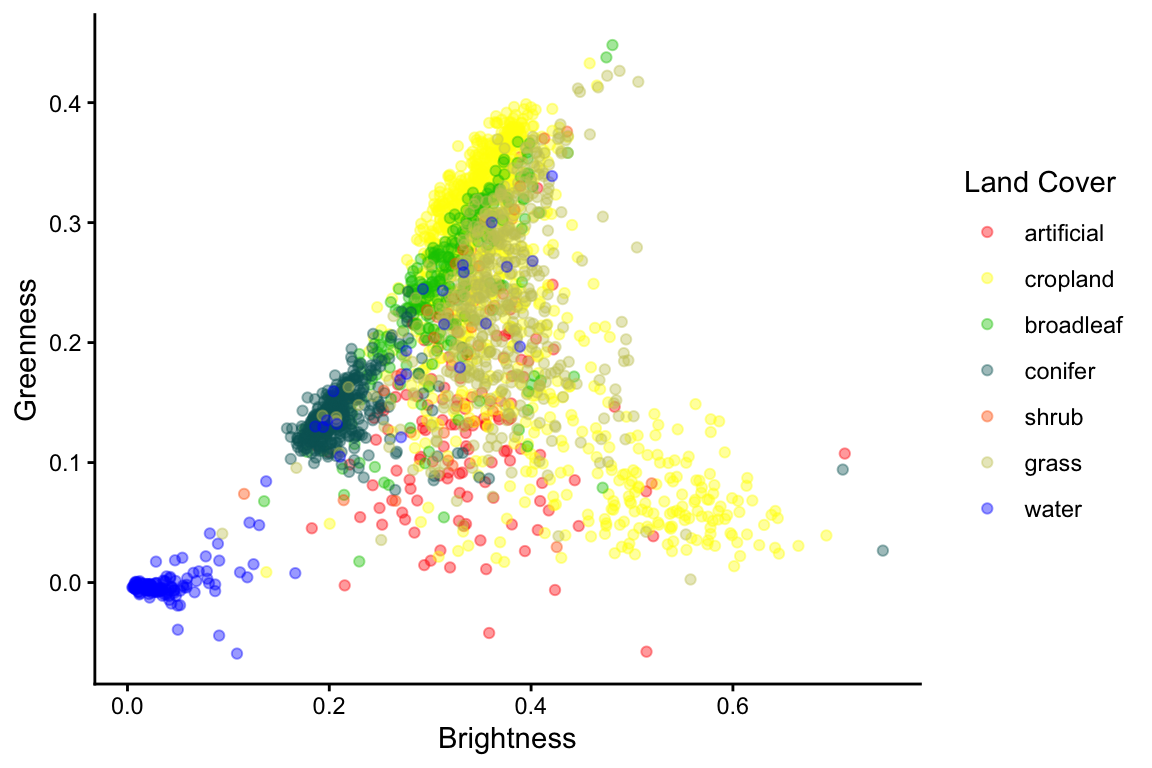
Classification
Train random forest
Random forest is implemented in the randomForest package and called with the randomForest() function (Breiman et al., 2022; Liaw and Wiener, 2002). We can use the familiar formula format to describe our response class and predictor variables. Multiple predictor variables are separated with a + sign.
myRfModel <- randomForest(class ~ band1 + band2 + band3, data=dataset)
Tip
Now it’s your turn to modify the formula so that the model predicts land cover using tasseled cap brightness, greenness, and wetness.
Printing the random forest model reveals information on the model, the out-of-bag error rate, and the confusion matrix. Note, the output below is based only on a small subset of the LUCAS samples. The out-of-bag error rate of the model below is 35%. Since \(Accuracy\) [%] = \(100 - Error\)[%], the classification accuracy is 65%.
rfm.lucas
Call:
 randomForest(formula = landcover ~ tcb + tcg + tcw, data = train_df[sample(nrow(train_df))[1:100],      ])
               Type of random forest: classification
                     Number of trees: 500
No. of variables tried at each split: 1

        OOB estimate of  error rate: 35%
Confusion matrix:
           artificial cropland broadleaf conifer shrub grass water class.error
artificial          2        2         2       0     0     0     0  0.66666667
cropland            1       18         3       0     0     7     0  0.37931034
broadleaf           1        2         7       1     0     2     1  0.50000000
conifer             0        0         1      23     0     0     0  0.04166667
shrub               0        0         0       0     0     0     1  1.00000000
grass               1        6         3       0     0     9     0  0.52631579
water               0        0         0       0     1     0     6  0.14285714
Evaluate model
We can plot the out-of-bag error against the number of trees to see if the model has converged:
plot(rfm.lucas)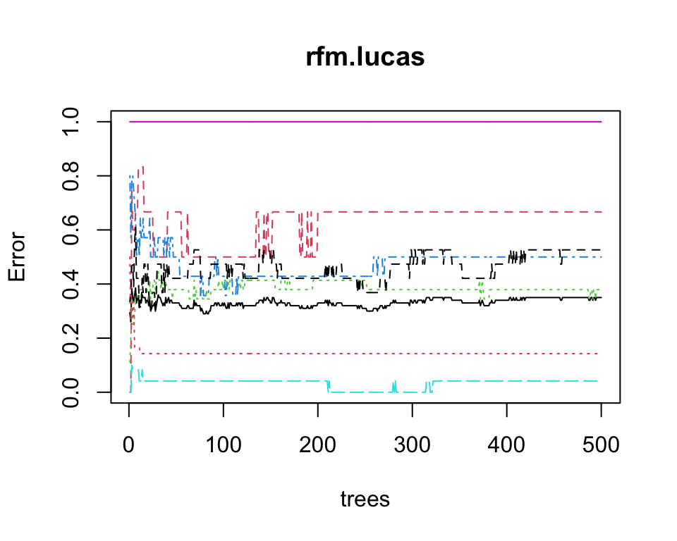
Validation
Estimates of map accuracy should be based on a probability sampling design (e.g. random or stratified random). If stratified random sampling is conducted with disproportional sampling (number of samples per class is disproportionate to the class area), then estimates must be corrected for sampling bias (Olofsson et al., 2014). In R, you can use the mapac package to accomplish this (Pflugmacher, 2021).
In our case, we have a systematic sample, which we may treat like a random sample. Hence, we can just create a confusion matrix and calculate the corresponding errors. Using table we can create the contingency-table (confusion matrix) between predicted and observed values. Here, we use the out-of-bag predictions from the random forest model.
# OOB predicted
lucas.oob.pred <- rfm.lucas$predicted

# LUCAS observations
lucas.oob.obs <- rfm.lucas$y

# Confusion matrix
conf <- table(lucas.oob.pred, lucas.oob.obs)
conf
lucas.oob.obs
lucas.oob.pred artificial cropland broadleaf conifer shrub grass water
artificial 2 1 1 0 0 1 0
cropland 2 18 2 0 0 6 0
broadleaf 2 3 7 1 0 3 0
conifer 0 0 1 23 0 0 0
shrub 0 0 0 0 0 0 1
grass 0 7 2 0 0 9 0
water 0 0 1 0 1 0 6conf <- table(lucas.oob.pred, lucas.oob.obs)
conf lucas.oob.obs
lucas.oob.pred artificial cropland broadleaf conifer shrub grass water
artificial 2 1 1 0 0 1 0
cropland 2 18 2 0 0 6 0
broadleaf 2 3 7 1 0 3 0
conifer 0 0 1 23 0 0 0
shrub 0 0 0 0 0 0 1
grass 0 7 2 0 0 9 0
water 0 0 1 0 1 0 6Overall accuracy:
sum(diag(conf)) / sum(conf)[1] 0.65User’s accuracy (1 - error of commission)
diag(conf) / apply(conf, 1, sum)artificial cropland broadleaf conifer shrub grass water
0.4000000 0.6428571 0.4375000 0.9583333 0.0000000 0.5000000 0.7500000 Producer’s accuracy (1 - error of omission)
diag(conf) / apply(conf, 2, sum)artificial cropland broadleaf conifer shrub grass water
0.3333333 0.6206897 0.5000000 0.9583333 0.0000000 0.4736842 0.8571429 Create map
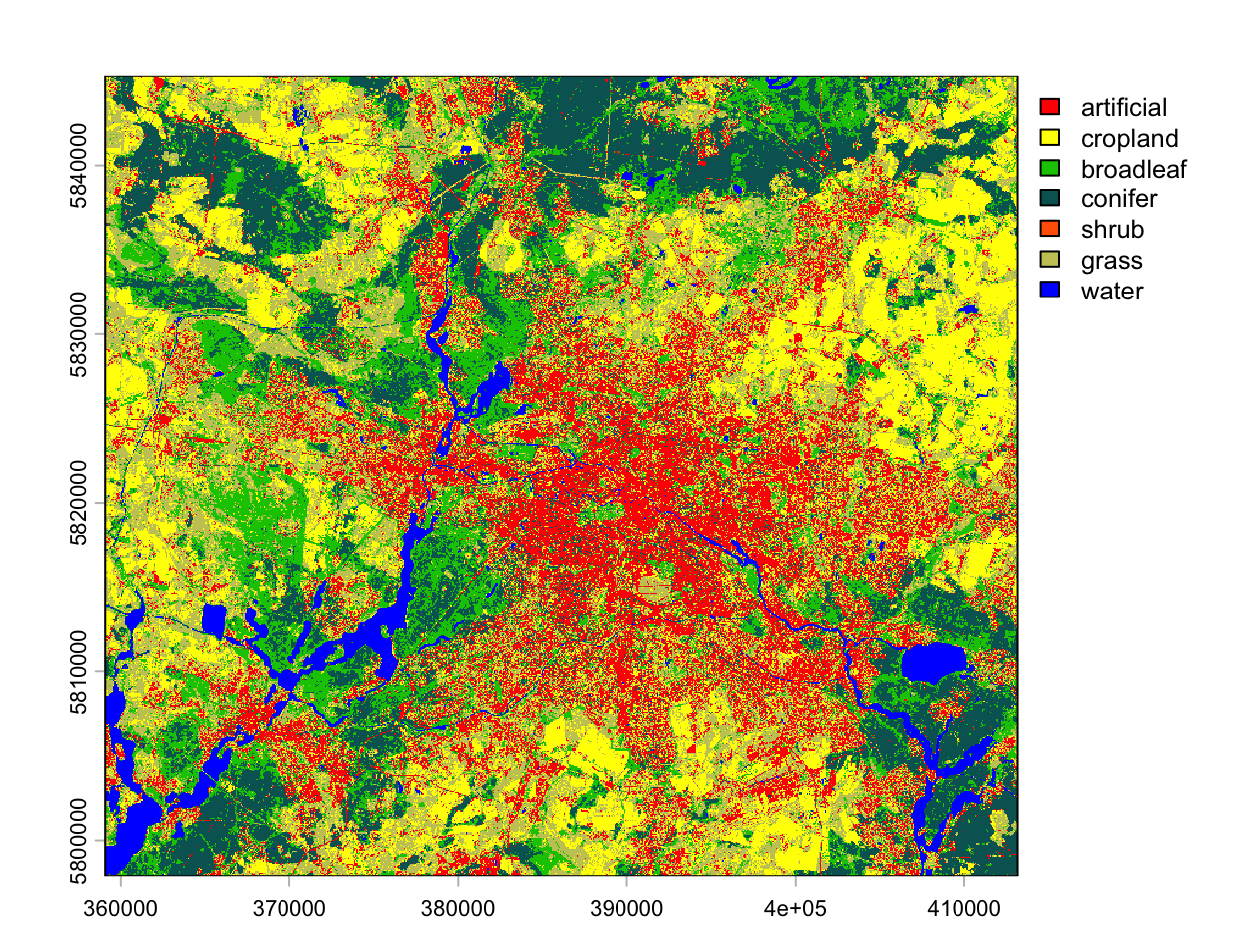
To create a land cover map, we need to apply the random forest model to the tasseled cap image. To save computing time, we do this on a spatial subset only.
myextent <- ext(c(359070, 413150, 5797900, 5845260)) # define extent object
l8tc_sub <- crop(l8tc, myextent)                     # crop image to extent
We can use the predict() function to apply the model to the image subset. This may take some time!
landcov_map <- predict(l8tc_sub, rfm.lucas)…and plot the prediction map using the RGB values from the legend file as class colors.
plot(landcov_map, col=lut$color, type="classes", levels=lut$label)