13 Principal Component Analysis

Background

Remote sensing data, especially high-dimensional data, often contain correlated variables. This means, that information that we seek to explain with them (e.g., vegetation cover gradients) may be shared by and distributed across multiple variables. Using transformations, we can create new variables that better describe the information in the data and also are uncorrelated.

Road to PCA

The basic aim of the principal component analysis is to transform a set of correlated variables, $B_1$, $B_2$, …, $B_n$, into a new set of uncorrelated variables, $Z_1$, $Z_2$, …, $Z_n$. The new variables are derived in decreasing order of “importance” in the sense that $Z_1$ accounts for as much of the variation in the original data. Then $Z_2$ is chosen to account for as much as possible of the remaining variation, subject to being uncorrelated with $Z1$, and so on. The new variables defined by this process, $Z_1$, $Z_2$, …, $Z_n$, are the principal components (Everitt, 2005).

Variance

Variance is a measure of the amount of variation or dispersion in a variable $X$. It is often written as $\sigma^2$ (to denote the unknown population variance) and $s^2$ (to denote the variance of a sample). Variance essentially is the mean of the squared differences between each observation $x_i$ and the mean $\bar x$ (Equation 13.1):

\[ s^2= \frac{1}{n-1} \sum_{i=1}^{n} (x_i - \bar x)^2 \tag{13.1}\]

Because variance is the squared difference, the units of the variance are also squared, e.g., $m^2$ for lengths/heights or $kg^2$ for weights. Thus, we need to take the square root, to obtain the original units: $s = \sqrt{s^2}$, where $s$ is called the standard deviation.

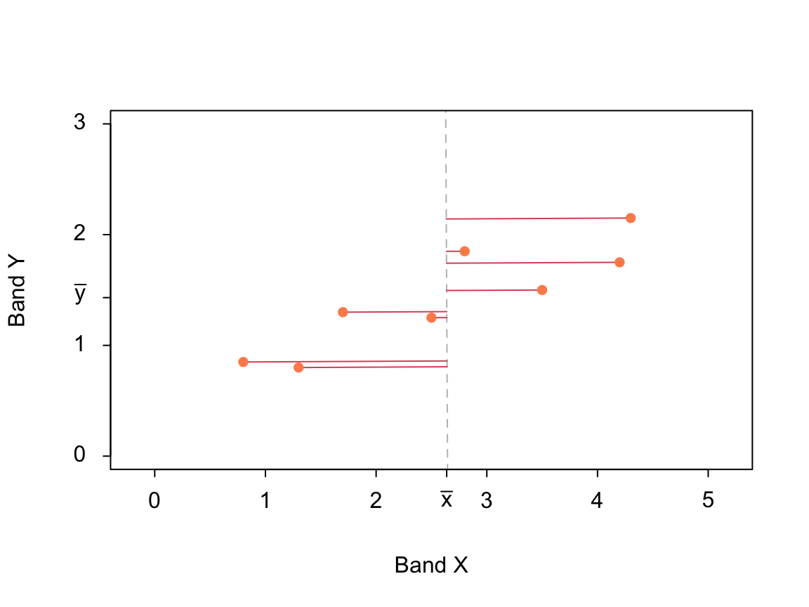
Let’s look at some made up dataset with variables $X$ and $Y$ (Figure 13.1). The vertical dashed grey line denotes the mean of $X$ $(\bar x)$. The horizontal red lines represent the differences between observations $(x_i)$ and their mean $(\bar x)$. Thus, the variance is the mean of the red lines’ lengths$^2$.

Figure 13.1: Scatterplot illustrating the variance of $X$

Covariance

Covariance is a measure of the joint variability of two random variables $X$ and $Y$, written as $s_{XY}$ or $cov(X,Y)$. You see the similarity to Equation 13.1, where we average $(x_i - \bar x)(x_i - \bar x)$.

\[ s_{XY}= \frac{1}{n-1} \sum_{i=1}^{n} (x_i - \bar x)*(y_i - \bar y) \tag{13.2}\]

Correlation

Correlation is the covariance standardized by the standard deviations of X and Y. It is often written as $\rho_{XY}$, $r$, or $cor(X,Y)$. As a result of the standardization, $\rho_{XY}$ always ranges between -1 and 1.

\[ r_{XY} = \frac{s_{XY}}{s_X s_Y} \tag{13.3}\]

Maximizing variance

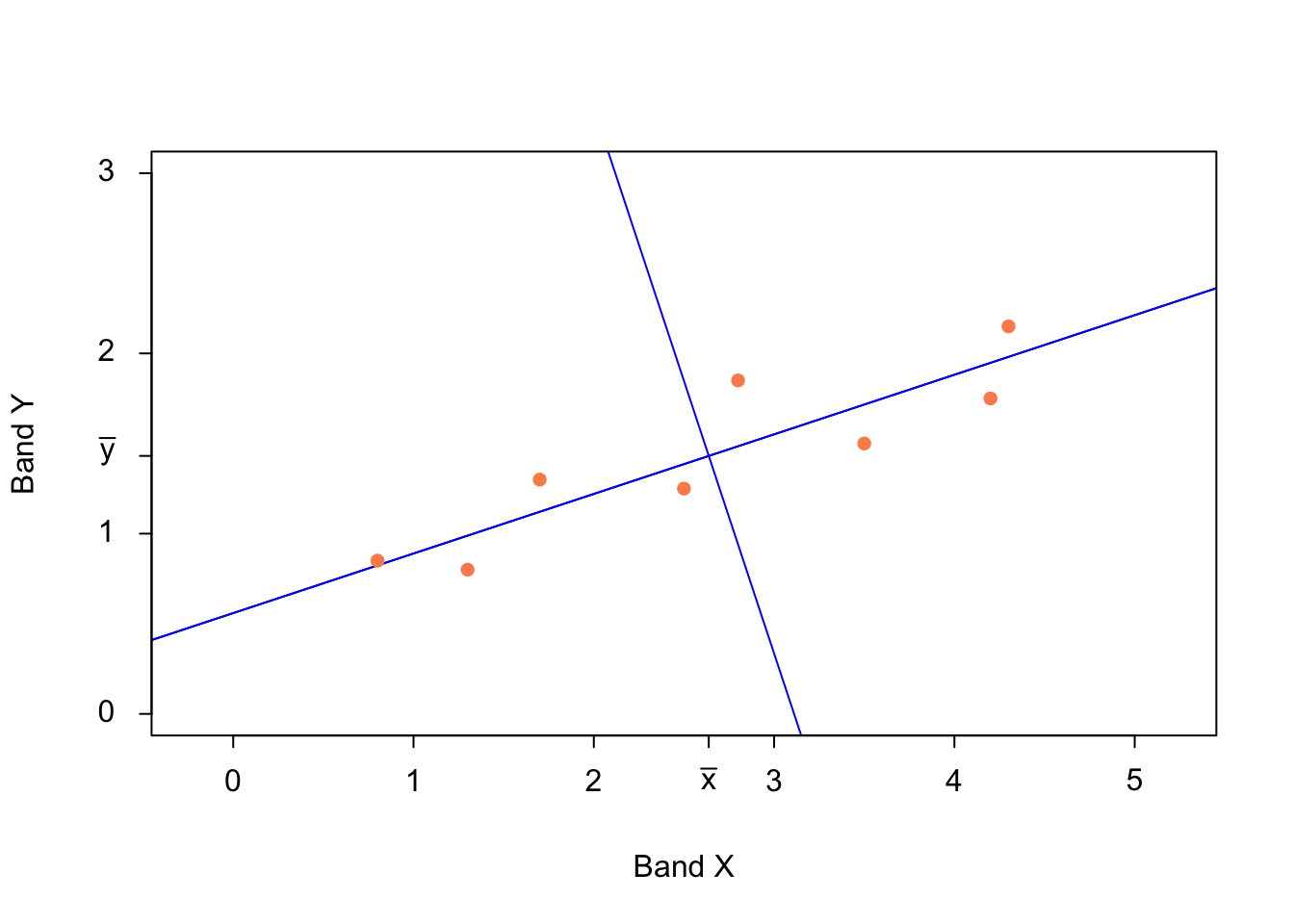
To find the first principal component of our dataset, we need to find a new coordinate axis that maximizes the variance. Let’s give this new axis (grey line) the letter $Z$. Axis $Z$ represents a new variable $Z$, which is just a transformation of our variables $X$ and $Y$, and it consists of observations $z_i$. In the graph below, mean $\bar z$ is represented by the dashed grey line, and the differences ($z_i - \bar z$) are the red lines. We rotate $Z$ until the variance $\sigma_Z^2$ is maximized. When that happens, $Z$ becomes the first principal component $PC1$ (blue line). Variance of $Z$, $s_Z^2 = \frac{1}{n-1} \sum_{i=1}^{n} (z_i - \bar z)^2$, is greater than $s_X^2$ and $s_Y^2$ and any other possible axis.

Maximizing variance (mean of the squared red lines).

It is interesting to see that, maximizing the variance minimizes the orthogonal distances at the same time (shown in light blue below). Note, this is different to the type of linear regression covered in session 2.2. Ordinary least squares regression minimizes the distances in the $y$ direction. PCA minimizes the distances perpendicular to the axis.

Maximizing variance (mean of the squared red lines).

Next axis please

A principal component analysis yields as many principal components (new axes) as there are orignal axes. In our example, we have two axes $X$ and $Y$, so we get two new axis $PC1$ and $PC2$. To find the next (second) principal component, we also search for the maximum variance, with the restriction that the next axis has to be orthogonal to the previous axis. Since, we have only two dimensions there is only one possible way to draw $PC2$.

Principal component axes in original data space

Data in transformed principal component space

PCA outputs

The principal component analysis yields two main outputs: 1) the eigenvalues, and 2) the eigenvectors. The eigenvalues represent the variances of the new axes. The eigenvectors describe the transformation coefficients. Similar to the tasseled cap coefficients, we can use the PCA coefficients to transform between original variables and principal components.

Summary

PCA yields a linear transformation of the original bands: the principal components (PC)

$PC_n = c_{n,1}X_1 + c_{n,1}X_2 + c_{n,1}X_1 + \dots + c_{n,n}X_n$

Unlike the Tasseled cap components, the principal components are not fixed; they can vary from scene to scene or dataset to dataset
However, PCA and Tasseled cap describe similar patterns in many landscapes
PCA is a method to derive principal components based on the variance of the input bands
The first n principal components contain most of the overall variance (feature reduction - compression)

Example data

WorldClim is a database of high spatial resolution global weather and climate data that can be used for mapping and spatial modeling. The bioclim dataset dervies from worldclim, i.e., from monthly temperature and rainfall values to generate more biologically meaningful variables. Bioclim are often used in species distribution modeling and related ecological modeling techniques. The original bioclim dataset contains 19 layers. For this demonstration, we’ll use a random sample collected over a geographic subset and only a subset of the variables:

BIO1 = Annual Mean Temperature
BIO5 = Max Temperature of Warmest Month
BIO6 = Min Temperature of Coldest Month
BIO12 = Annual Precipitation

clim <- read.csv("data/landcov/bioclim_subset_sample.csv")
head(clim)

      Tmean     Tmax      Tmin   Precip
1  8.483958 21.75500 -7.096000 705.5000
2  6.497375 20.52900 -9.607000 749.0000
3 10.452375 24.45300 -5.697000 660.5000
4  8.237074 22.02089 -8.008889 637.1111
5  8.276444 21.41000 -6.908667 621.8333
6 11.461416 25.75200 -4.883000 684.2500

A look at the scatter plot matrix shows that Tmean and Tmax are strongly correlated with each other and that both variables are also correlated to some degree with Tmin. If we were to use these four variables in a regression model, we would face the issue of multicollinearity. Statistical inference for regression models hat contain intercorrelations among two or more independent variables is less reliable as multicolinearity leads to wider confidence intervals. In this case, it will likely be difficult to tell whether an effect is due to Tmean or Tmax. One way to reduce multicollinearity is to eliminate variables based on correlation coefficients or scientific knowledge. Often this is an effective approach if there is prior knowledge regarding the variables, but it can be cumbersome for larger sets of predictors. Another approach is the principal component analysis, which reduces the dimensionality (less predictors are needed) and it yields uncorrelated predictors.

pairs(clim)

Fit PCA

There are two functions in R for performing a PCA: princomp() and prcomp(). While the former function calculates the eigenvalue on the correlation/co-variance matrix using the function eigen(), the latter function uses singular value decomposition, which numerically more stable. We here are going to use prcomp().

pca <- prcomp(clim, center = T, scale. = TRUE)

You should set the center and scale. argument to TRUE, to transform the data matrix to mean zero and unit variance. The default is scale. = FALSE. You may also use scale() to standardize the original data matrix and then enter the standardized data matrix to prcomp.

Scores

The prcomp object stores the transformation and the transformed values, which are called scores. You can access the transformed dataset as follows:

pca_scores <- data.frame(pca$x)
head(pca_scores)

          PC1        PC2        PC3         PC4
1 -0.10437038 -0.6623921  0.5218369 -0.06333806
2 -1.81424024  0.2309886 -0.1090850  0.02493079
3  1.57278761 -1.0321770  0.4015154  0.02441915
4 -0.19815948  0.1256635  0.3803971 -0.05908909
5  0.06685627 -0.2714205  1.0023861 -0.04971012
6  2.30800977 -1.5264628  0.2270009  0.07219499

You see the transformed variables (now called PC1, PC2, PC3, PC4) are uncorrelated.

pairs(pca_scores)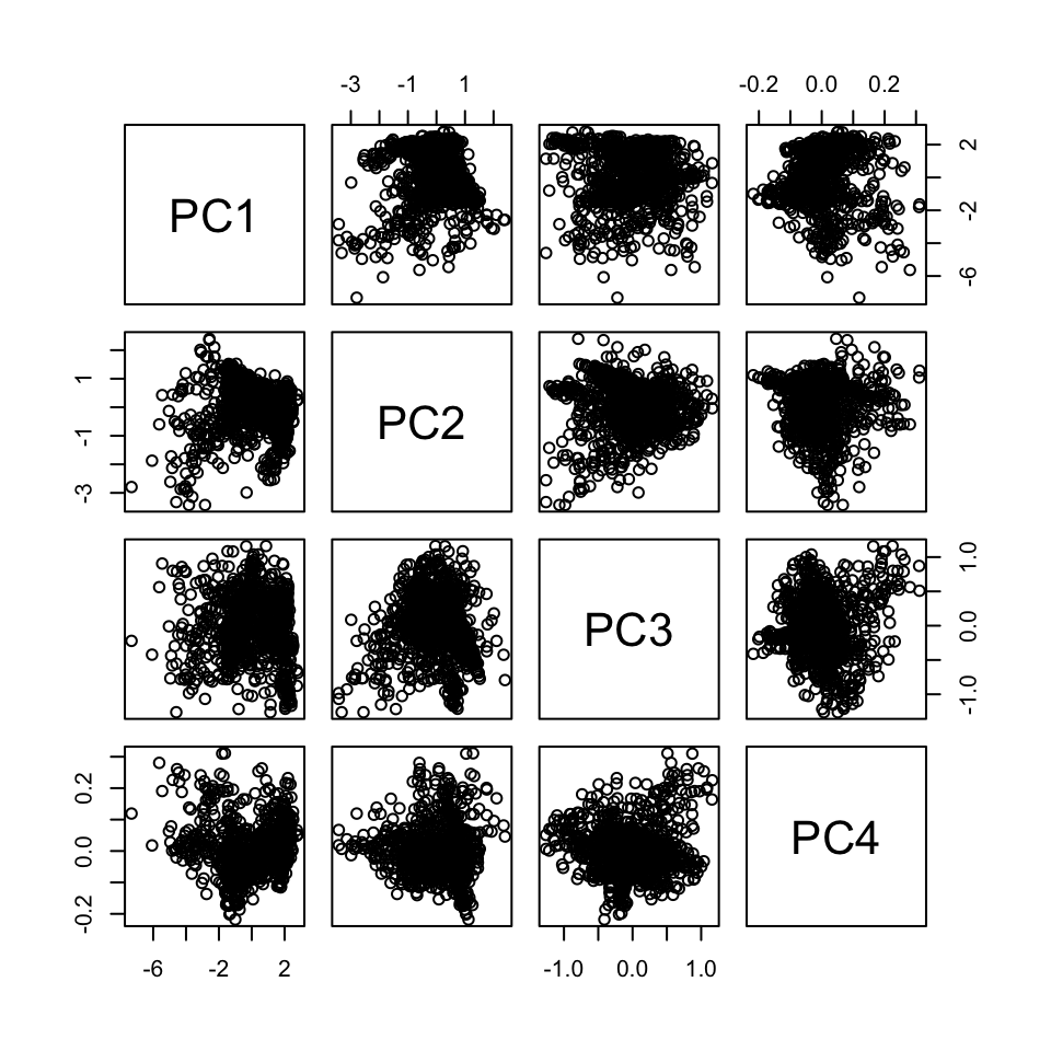

You can apply the transformation (rotation coefficients) to a dataset using the predict function. In the example below, the transformation is applied to the same dataset that was used to fit the transformation. Hence, the results are the same as the scores stored in the prcomp object (pca$x).

predicted_pca_scores <- predict(pca, clim)
head(predicted_pca_scores)

             PC1        PC2        PC3         PC4
[1,] -0.10437038 -0.6623921  0.5218369 -0.06333806
[2,] -1.81424024  0.2309886 -0.1090850  0.02493079
[3,]  1.57278761 -1.0321770  0.4015154  0.02441915
[4,] -0.19815948  0.1256635  0.3803971 -0.05908909
[5,]  0.06685627 -0.2714205  1.0023861 -0.04971012
[6,]  2.30800977 -1.5264628  0.2270009  0.07219499

Rotation coefficients

The PCA transformation consists of rotation coefficients (eigenvectors). You can access the rotation coefficients stored in a prcomp object as follows:

pca$rotation

              PC1        PC2        PC3         PC4
Tmean   0.5671218 -0.1334564 -0.2842325 -0.76142902
Tmax    0.5561077  0.0899659 -0.5600202  0.60747649
Tmin    0.4561343 -0.6196440  0.5977105  0.22522181
Precip -0.4013209 -0.7682036 -0.4983286  0.02175513

Recall, the coefficients describe how each PC is a linear combination of the input variables. An interesting analogy is a cooking recipe. The cooking recipe below defines the fractions of the climate variables that are needed (and added up) to “cook up” the first principal component.

\[ PC1 = 0.567 * Tmean + 0.556 * Tmax + 0.456 * Tmin + -0.401 *Precip \]

Let’s do this calculation for the first observation in our bioclim dataset. Note, that below I scale the variables to unit variance and mean zero (z-score). When running the principal component analysis above, I set the scale argument of the prcomp function to TRUE, which has the same effect.

# first observation
clim_obs <- head(scale(clim),1)
clim_obs

           Tmean       Tmax      Tmin    Precip
[1,] -0.07088585 -0.4483495 0.6604827 0.2893138

# rotation coefficients of the first PC
pca1_coeff <- pca$rotation[,1]
pca1_coeff

     Tmean       Tmax       Tmin     Precip 
 0.5671218  0.5561077  0.4561343 -0.4013209

Multiplying the observation vector and the coefficient vector is a vectorized operation. That is, the first element of the first vector is multiplied with the first element of the second vector, the second element of the first vector is multiplied with the second element of the second vector, etc.

sum(clim_obs * pca1_coeff)

[1] -0.1043704

We just calculated the score of the first principal component (PC1) for a single observation. The PC1 is a transformation (the cooking recipe) and the score is the value you get when applying the transformation. Let’s compare our score with the one obtained with prcomp.

head(pca$x, 1)

            PC1        PC2       PC3         PC4
[1,] -0.1043704 -0.6623921 0.5218369 -0.06333806

So, the coefficients reflect the contribution of each variable to each principal component. For example, the absolute magnitude of the $PC1$ coefficients for $Tmean$, $Tmax$, $Tmin$, and $Precip$ is relatively similar, which indicates that all four variables contribute (roughly) similarly to PC1.

The sign of the coefficients tells us something about the direction, i.e., $PC1$ increases with increasing $Precip$, whereas $PC1$ decreases with increasing $Tmean$, $Tmax$, and $Tmin$. Note, however, the direction of the eigenvector is arbitrary. The equation below flips the signs of the coefficients (direction of the eigenvector). The inverse: $-1 * PC1$ is equally valid:

\[ PC_i \hat{=} -PC_i \]

So, do not get attached to the direction of the PC1. But what the signs tell us is: $Tmean$, $Tmax$, and $Tmin$ have an opposite sign to $Precip$. We can also say: $Tmean$, $Tmax$, and $Tmin$ form a contrast to $Precip$ (while one has a positive effect the other has a negative effect or vice versa). Now, to interpret what that means requires scientific knowledge of the underlying ecological, climatological, biological, or socio-ecological gradients you might be observing here, e.g. elevation gradients, continentality, etc.

Eigenvalues

To explore how the total variance of our four climate variables is now re-partitioned in the derived principal components, we need to take a look a the eigenvalues. Recall, the eigenvalues are the variances explained by the principal components (one for each component). The square roots of the eigenvalues are stored in the prcomp object:

pca$sdev

[1] 1.73331374 0.88945906 0.44527838 0.07882397

From this, we can easily calculate the variance explained by each component (the component variance divided by the total variance).

var_exp <- data.frame(pc = 1:4,
                      var_exp = pca$sdev^2 / sum(pca$sdev^2))

# add the variances cumulatively
var_exp$var_exp_cumsum <- cumsum(var_exp$var_exp)
var_exp

  pc     var_exp var_exp_cumsum
1  1 0.751094132      0.7510941
2  2 0.197784356      0.9488785
3  3 0.049568208      0.9984467
4  4 0.001553304      1.0000000

The so called scree plot plots the component variances versus the component number. The idea is to look for an “elbow” which corresponds to the point after which the eigenvalues decrease more slowly.

par(mfrow=c(1,2))
plot(var_exp$pc, var_exp$var_exp, type="b", col=4,
     ylab="Fraction of explained variance", xlab="Principal Component")
plot(var_exp$pc, var_exp$var_exp_cumsum, type="b", col=6,
     ylab="Cummulative fraction variance", xlab="Principal Component")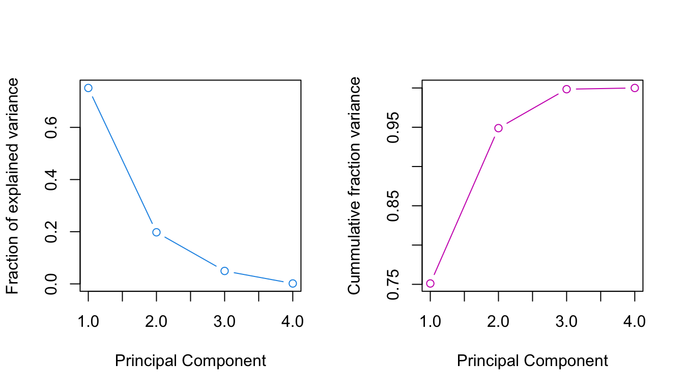

You are probably not surprised there is an easier way:

summary(pca)

Importance of components:
                          PC1    PC2     PC3     PC4
Standard deviation     1.7333 0.8895 0.44528 0.07882
Proportion of Variance 0.7511 0.1978 0.04957 0.00155
Cumulative Proportion  0.7511 0.9489 0.99845 1.00000

The eigenvalues tell us: 75.1% of the variance is explained by PC1 alone, 19.8% by PC2, 5% by PC3, and only 0.16% by PC4. The cumulative proportion makes clear that 99.8% of the variance is captured by the first three components. Hence, we may discard PC4 without loosing much information.

Correlation analysis

Another way to interpret the meaning of the principal components is to explore the correlation between the PC scores and the original variables. Explore the scatter plot below and look at how PC1 is correlated with the orginal variables. Compare this to your observation of the rotation coefficients. You can do the same for PC2, PC3, and PC4.

df <- cbind(clim, pca_scores)
pairs(df[,1:7])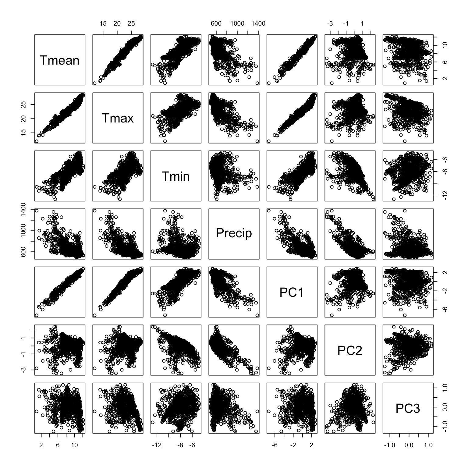

Biplot

The biplot shows the bioclim variables (in form of the rotation coefficients / loadings) and the observations (the PCA scores of our 10k samples) in one graphic. The variables are visualized as arrows from the plot origin, reflecting their direction and magnitude. Note, there are different versions of biplots out there also in different packages (e.g. PCAtools, ggbiplot).

biplot(pca)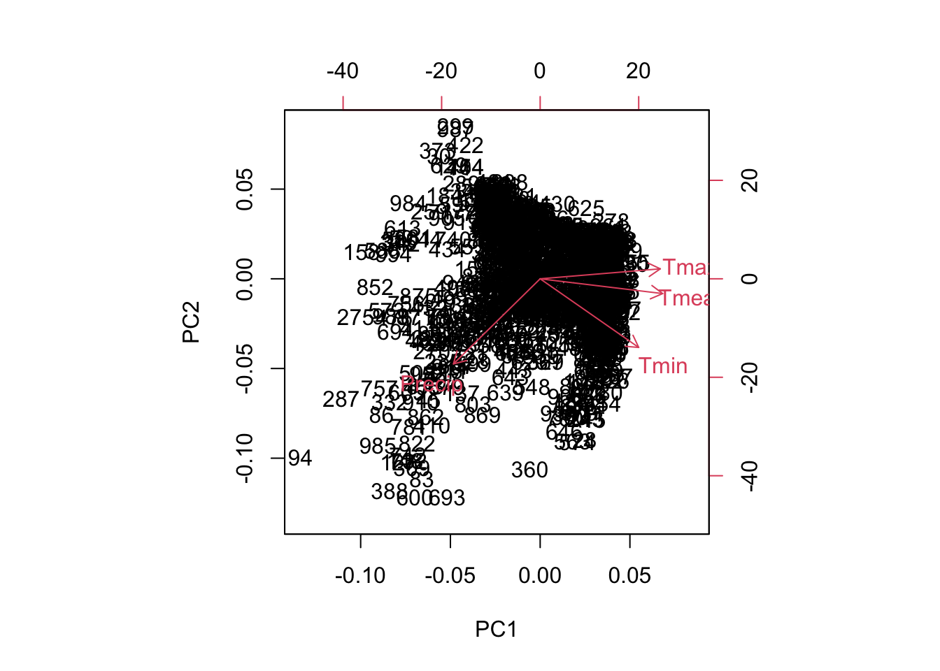

biplot(pca, choices=c(1,3))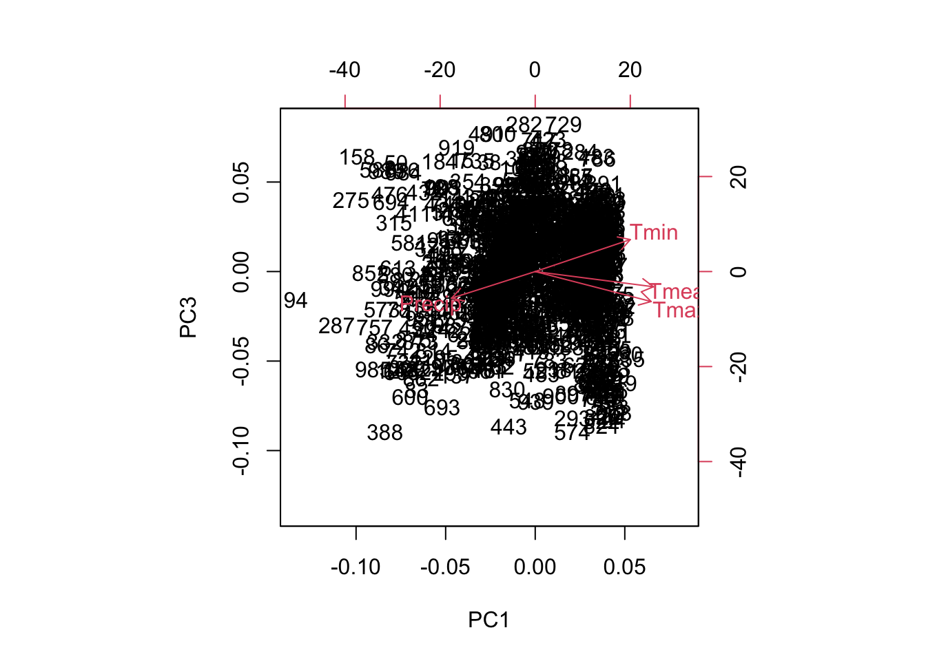

biplot(pca, choices=c(1,3), xlabs=rep('.', nrow(pca$x)))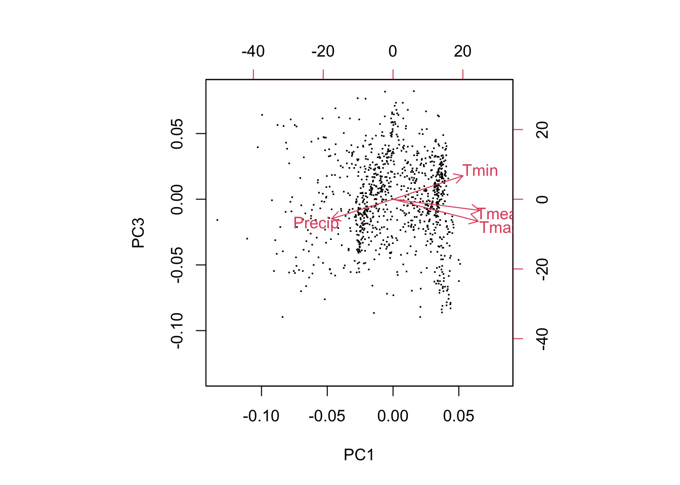

`prcomp` vs `princomp`

Description	prcomp()	princomp()
Decomposition method	svd()	eigen()
Standard deviations of the principal components	sdev	sdev
Matrix of variable loadings (columns are eigenvectors)	rotation	loadings
Variable means (means that were substracted)	center	center
Variable standard deviations (the scalings applied to each variable )	scale	scale
Coordinates of observations on the principal components	x	scores