library(MuMIn) # also exhaustive model searching17 Model selection
Packages
Data tranformations
Sometimes the relationship between two variables is not linear, which makes the linear model unsuitable. You also see below that the variance in Ozone increases with increasing Temperature (heteroscedasticity), which also violates the assumption of homogeneous variance for the linear regression model.
data("airquality")
plot(airquality$Temp, airquality$Ozone, cex=.8,
     xlab='Temperature [K]', ylab='Ozone [ppm]')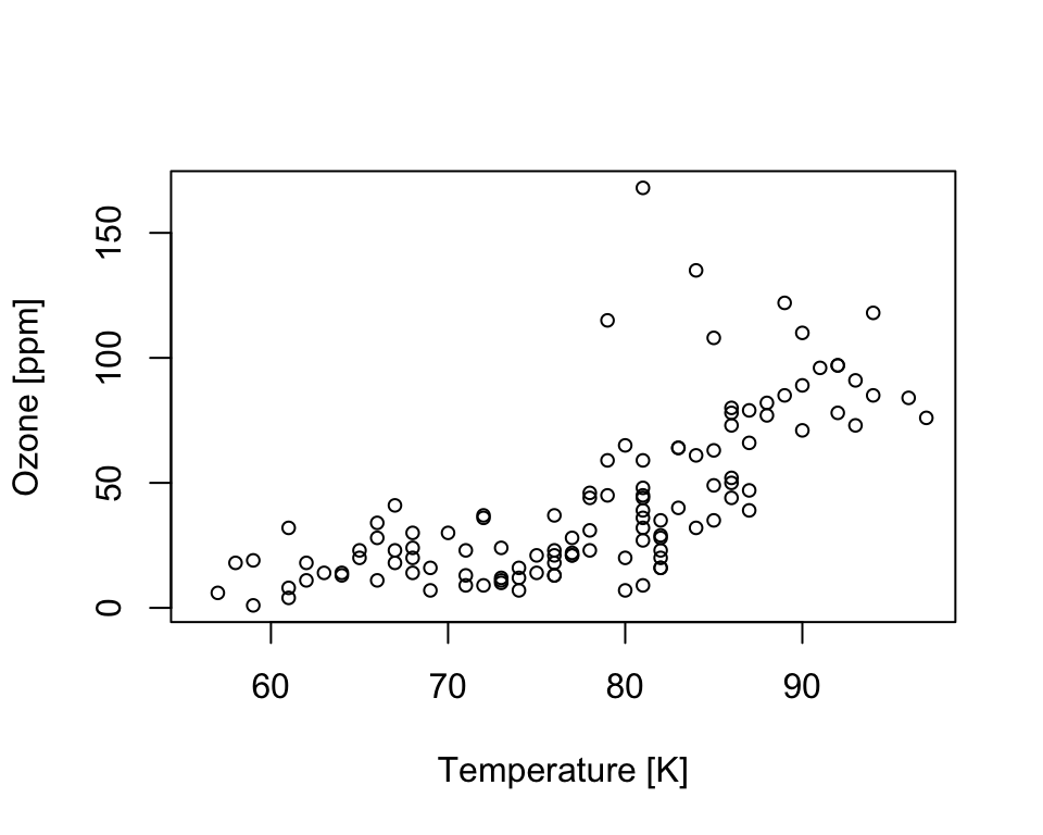
Transforming the response variable (here with a log-transformation) can linearize the relationship and homogenize the variance.
lmd <- lm(log(Ozone) ~ Temp, data=airquality)

plot(airquality$Temp, log(airquality$Ozone), cex=.8,
     xlab='Temperature [K]', ylab='log-Ozone [ppm]')
abline(lmd, col='blue')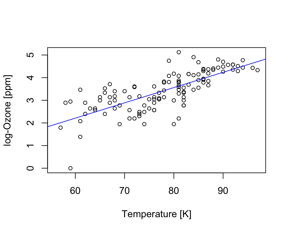
Example data
We will illustrate the variable selection method on data from 50 U.S. states. The variables are population estimate as of July 1, 1975, per capita income (1974), illiteracy (1970, percent of population), life expectancy in years (1969-71), murder and non-negligent manslaughter rate per 100,000 population (1976), percent high-school graduates (1970), mean number of days with min temperature 32 degrees (1931- 1960) in capital or large city, and land area in square miles. The data was collected from US Bureau of the Census. We will take life expectancy as the response and the remaining variables as predictors. Example and most text is taken from Faraway (2002).
data("state")
names(state.x77)NULL# a fix is necessary to remove spaces in some of the variable names
statedata <- data.frame(state.x77, row.names=state.abb, check.names=T)
head(statedata) Population Income Illiteracy Life.Exp Murder HS.Grad Frost Area
AL 3615 3624 2.1 69.05 15.1 41.3 20 50708
AK 365 6315 1.5 69.31 11.3 66.7 152 566432
AZ 2212 4530 1.8 70.55 7.8 58.1 15 113417
AR 2110 3378 1.9 70.66 10.1 39.9 65 51945
CA 21198 5114 1.1 71.71 10.3 62.6 20 156361
CO 2541 4884 0.7 72.06 6.8 63.9 166 103766Selection criteria
Model selection is the process of selecting a model from a set of candidate models. To do this, we need to define potential selection criteria. Selection techniques based on probabilistic measures balance the goodness of fit with model simplicity (parsimonious models). If models include too many predictors, they may poorly generalize (overfitting) and the may be harder to interpret. Selection criteria based purely on model performance can also avoid overfitting (they incorporate cross-validation), but model complexity is not so much of a concern than there is prediction performance.
AIC
If there are p potential predictors, then there are 2\(p\) possible models. We fit all these models and choose the best one according to some criterion. The Akaike Information Criterion (AIC) and the Bayes Information Criterion (BIC) are some other commonly used criteria.
\[AIC = -2*log - likelihood + 2 p \tag{17.1}\]
For linear regression models, the -2log-likelihood (known as the deviance is n*log(RSS/n) . We want to minimize AIC. Larger models will fit better and so have smaller RSS (residual sum of squares) but use more parameters. Thus the best choice of model will balance fit with model size.
Model search
There are different techniques for searching potential model candidates. The most well known (and oldest) technique is stepwise regression. Here, models are developed by iteratively adding and/or removing predictor variables. For example, one can start with a full model (all predictor variables) and remove predictors one at a time until the search criterium is met (backwards elimination). Or, one could start with a null model (no predictors) and add predictors (one at a time) until the search criterium is met (forward selection). Stepwise regression can be effective, but it can be quite blind to certain predictor combinations. Simply, because the technique can only see one step ahead or back. With modern computing power it is often (not always) possible to fit all variable combinations and pick the best according to a search criterium.
All subset regression tests all possible subsets of the set of potential predictor variables. If there are K potential predictor variables (besides the constant), then there are \(2^k\) distinct subsets of them to be tested. In R we can use the MuMIn() package to do exhaustive model search (Bartoń, 2022). There are other packages as well, e.g., bestglm, leaps.
To search through all possible variable combinations, we provide dredge() with a full model (the most complex model). Model complexity is defined here as the number of parameters. The result is a list of all potential models ranked by the defined selection criterium, e.g. AIC. We must keep in mind, that we are just operating on a sample, and that it is likely that there is no single best model. Picking the second or third best model is fine when it is simpler and/or there is scientific reason to to so.
Note, the dot (.) in the model formula means all remaining variables (in the data.frame) are used predictors.
options(na.action='na.fail')

lm.full <- lm(Life.Exp ~ ., data=statedata)
lm.all <- dredge(lm.full, rank='AIC')
lm.all
Fixed term is "(Intercept)"| (Intercept) | Area | Frost | HS.Grad | Illiteracy | Income | Murder | Population | df | logLik | AIC | delta | weight | |
|---|---|---|---|---|---|---|---|---|---|---|---|---|---|
| 103 | 71.027 | NA | -0.006 | 0.047 | NA | NA | -0.300 | 0 | 6 | -51.866 | 115.733 | 0.000 | 2.313360e-01 |
| 119 | 71.066 | NA | -0.006 | 0.048 | NA | 0.000 | -0.300 | 0 | 7 | -51.860 | 117.720 | 1.987 | 8.565862e-02 |
| 111 | 70.950 | NA | -0.006 | 0.047 | 0.029 | NA | -0.302 | 0 | 7 | -51.862 | 117.724 | 1.992 | 8.546254e-02 |
| 104 | 71.005 | 0 | -0.006 | 0.047 | NA | NA | -0.299 | 0 | 7 | -51.865 | 117.731 | 1.998 | 8.517589e-02 |
| 39 | 71.036 | NA | -0.007 | 0.050 | NA | NA | -0.283 | NA | 5 | -53.987 | 117.974 | 2.242 | 7.541813e-02 |
| 55 | 70.837 | NA | -0.007 | 0.044 | NA | 0.000 | -0.286 | NA | 6 | -53.807 | 119.614 | 3.881 | 3.322657e-02 |
| 47 | 71.520 | NA | -0.008 | 0.045 | -0.182 | NA | -0.273 | NA | 6 | -53.817 | 119.634 | 3.902 | 3.288256e-02 |
| 127 | 70.989 | NA | -0.006 | 0.048 | 0.028 | 0.000 | -0.302 | 0 | 8 | -51.856 | 119.712 | 3.979 | 3.163943e-02 |
| 112 | 70.887 | 0 | -0.006 | 0.048 | 0.037 | NA | -0.301 | 0 | 8 | -51.859 | 119.719 | 3.986 | 3.152667e-02 |
| 120 | 71.056 | 0 | -0.006 | 0.048 | NA | 0.000 | -0.300 | 0 | 8 | -51.860 | 119.719 | 3.987 | 3.151601e-02 |
| 40 | 70.913 | 0 | -0.007 | 0.052 | NA | NA | -0.279 | NA | 6 | -53.962 | 119.924 | 4.191 | 2.845750e-02 |
| 101 | 70.415 | NA | NA | 0.041 | NA | NA | -0.266 | 0 | 5 | -55.009 | 120.017 | 4.285 | 2.715352e-02 |
| 109 | 69.552 | NA | NA | 0.053 | 0.396 | NA | -0.302 | 0 | 6 | -54.009 | 120.018 | 4.286 | 2.713802e-02 |
| 63 | 71.285 | NA | -0.008 | 0.040 | -0.160 | 0.000 | -0.277 | NA | 7 | -53.676 | 121.353 | 5.620 | 1.392781e-02 |
| 56 | 70.628 | 0 | -0.007 | 0.046 | NA | 0.000 | -0.279 | NA | 7 | -53.749 | 121.499 | 5.766 | 1.294629e-02 |
| 110 | 69.122 | 0 | NA | 0.060 | 0.430 | NA | -0.292 | 0 | 7 | -53.770 | 121.540 | 5.807 | 1.268250e-02 |
| 48 | 71.489 | 0 | -0.008 | 0.045 | -0.178 | NA | -0.273 | NA | 7 | -53.817 | 121.633 | 5.901 | 1.210441e-02 |
| 128 | 70.943 | 0 | -0.006 | 0.049 | 0.034 | 0.000 | -0.301 | 0 | 9 | -51.855 | 121.709 | 5.977 | 1.165307e-02 |
| 102 | 70.200 | 0 | NA | 0.045 | NA | NA | -0.259 | 0 | 6 | -54.922 | 121.844 | 6.112 | 1.089239e-02 |
| 117 | 70.576 | NA | NA | 0.045 | NA | 0.000 | -0.267 | 0 | 6 | -54.923 | 121.846 | 6.113 | 1.088440e-02 |
| 125 | 69.684 | NA | NA | 0.056 | 0.389 | 0.000 | -0.302 | 0 | 7 | -53.963 | 121.926 | 6.193 | 1.045762e-02 |
| 115 | 72.274 | NA | -0.006 | NA | NA | 0.000 | -0.331 | 0 | 6 | -55.354 | 122.707 | 6.974 | 7.075805e-03 |
| 51 | 71.989 | NA | -0.007 | NA | NA | 0.000 | -0.317 | NA | 5 | -56.575 | 123.149 | 7.417 | 5.672035e-03 |
| 108 | 74.244 | 0 | -0.008 | NA | -0.423 | NA | -0.324 | 0 | 7 | -54.607 | 123.214 | 7.482 | 5.490947e-03 |
| 100 | 73.731 | 0 | -0.006 | NA | NA | NA | -0.362 | 0 | 6 | -55.649 | 123.298 | 7.566 | 5.264349e-03 |
| 64 | 71.120 | 0 | -0.007 | 0.042 | -0.140 | 0.000 | -0.274 | NA | 8 | -53.663 | 123.325 | 7.592 | 5.194776e-03 |
| 59 | 72.866 | NA | -0.008 | NA | -0.400 | 0.000 | -0.288 | NA | 6 | -55.716 | 123.433 | 7.700 | 4.922729e-03 |
| 126 | 69.202 | 0 | NA | 0.061 | 0.425 | 0.000 | -0.293 | 0 | 8 | -53.762 | 123.523 | 7.790 | 4.705026e-03 |
| 107 | 74.188 | NA | -0.007 | NA | -0.433 | NA | -0.306 | 0 | 6 | -55.782 | 123.565 | 7.832 | 4.608228e-03 |
| 99 | 73.662 | NA | -0.005 | NA | NA | NA | -0.344 | 0 | 5 | -56.824 | 123.648 | 7.915 | 4.419940e-03 |
| 123 | 72.897 | NA | -0.007 | NA | -0.304 | 0.000 | -0.307 | 0 | 7 | -54.865 | 123.731 | 7.998 | 4.241552e-03 |
| 118 | 70.372 | 0 | NA | 0.048 | NA | 0.000 | -0.260 | 0 | 7 | -54.870 | 123.739 | 8.007 | 4.223192e-03 |
| 37 | 70.297 | NA | NA | 0.044 | NA | NA | -0.237 | NA | 4 | -57.984 | 123.968 | 8.236 | 3.765969e-03 |
| 116 | 72.670 | 0 | -0.006 | NA | NA | 0.000 | -0.345 | 0 | 7 | -54.986 | 123.972 | 8.239 | 3.759389e-03 |
| 44 | 74.619 | 0 | -0.009 | NA | -0.596 | NA | -0.297 | NA | 6 | -56.103 | 124.207 | 8.474 | 3.342471e-03 |
| 43 | 74.557 | NA | -0.009 | NA | -0.602 | NA | -0.280 | NA | 5 | -57.147 | 124.295 | 8.562 | 3.198912e-03 |
| 124 | 73.459 | 0 | -0.008 | NA | -0.349 | 0.000 | -0.320 | 0 | 8 | -54.346 | 124.692 | 8.959 | 2.622760e-03 |
| 60 | 73.294 | 0 | -0.009 | NA | -0.443 | 0.000 | -0.296 | NA | 7 | -55.415 | 124.829 | 9.097 | 2.448596e-03 |
| 52 | 72.209 | 0 | -0.007 | NA | NA | 0.000 | -0.324 | NA | 6 | -56.443 | 124.887 | 9.154 | 2.379538e-03 |
| 97 | 72.893 | NA | NA | NA | NA | NA | -0.312 | 0 | 4 | -58.545 | 125.089 | 9.356 | 2.150330e-03 |
| 45 | 69.735 | NA | NA | 0.052 | 0.254 | NA | -0.258 | NA | 5 | -57.610 | 125.221 | 9.488 | 2.013488e-03 |
| 38 | 69.931 | 0 | NA | 0.050 | NA | NA | -0.224 | NA | 5 | -57.750 | 125.500 | 9.767 | 1.750954e-03 |
| 113 | 71.754 | NA | NA | NA | NA | 0.000 | -0.298 | 0 | 5 | -57.760 | 125.520 | 9.787 | 1.733755e-03 |
| 53 | 70.142 | NA | NA | 0.039 | NA | 0.000 | -0.239 | NA | 5 | -57.898 | 125.796 | 10.064 | 1.509800e-03 |
| 98 | 72.847 | 0 | NA | NA | NA | NA | -0.320 | 0 | 5 | -58.001 | 126.001 | 10.269 | 1.362806e-03 |
| 46 | 69.146 | 0 | NA | 0.062 | 0.305 | NA | -0.246 | NA | 6 | -57.224 | 126.447 | 10.715 | 1.090328e-03 |
| 35 | 73.900 | NA | -0.006 | NA | NA | NA | -0.328 | NA | 4 | -59.258 | 126.516 | 10.784 | 1.053440e-03 |
| 36 | 73.970 | 0 | -0.007 | NA | NA | NA | -0.344 | NA | 5 | -58.261 | 126.523 | 10.790 | 1.050117e-03 |
| 61 | 69.483 | NA | NA | 0.046 | 0.276 | 0.000 | -0.262 | NA | 6 | -57.463 | 126.926 | 11.193 | 8.584254e-04 |
| 105 | 72.907 | NA | NA | NA | -0.041 | NA | -0.307 | 0 | 5 | -58.532 | 127.064 | 11.332 | 8.010028e-04 |
| 54 | 69.666 | 0 | NA | 0.045 | NA | 0.000 | -0.225 | NA | 6 | -57.597 | 127.194 | 11.462 | 7.505926e-04 |
| 114 | 71.981 | 0 | NA | NA | NA | 0.000 | -0.306 | 0 | 6 | -57.631 | 127.263 | 11.530 | 7.252955e-04 |
| 121 | 71.615 | NA | NA | NA | 0.087 | 0.000 | -0.308 | 0 | 6 | -57.710 | 127.420 | 11.688 | 6.703066e-04 |
| 49 | 71.226 | NA | NA | NA | NA | 0.000 | -0.270 | NA | 4 | -59.834 | 127.668 | 11.935 | 5.923061e-04 |
| 62 | 68.675 | 0 | NA | 0.056 | 0.347 | 0.000 | -0.249 | NA | 7 | -56.935 | 127.871 | 12.138 | 5.350955e-04 |
| 106 | 72.848 | 0 | NA | NA | -0.005 | NA | -0.320 | 0 | 6 | -58.000 | 128.001 | 12.268 | 5.014273e-04 |
| 122 | 71.846 | 0 | NA | NA | 0.081 | 0.000 | -0.315 | 0 | 7 | -57.589 | 129.177 | 13.445 | 2.784771e-04 |
| 33 | 72.974 | NA | NA | NA | NA | NA | -0.284 | NA | 3 | -61.642 | 129.285 | 13.552 | 2.639198e-04 |
| 57 | 71.164 | NA | NA | NA | 0.037 | 0.000 | -0.274 | NA | 5 | -59.826 | 129.651 | 13.919 | 2.196954e-04 |
| 50 | 71.228 | 0 | NA | NA | NA | 0.000 | -0.270 | NA | 5 | -59.834 | 129.668 | 13.935 | 2.179018e-04 |
| 34 | 72.936 | 0 | NA | NA | NA | NA | -0.290 | NA | 4 | -61.299 | 130.598 | 14.866 | 1.368276e-04 |
| 41 | 73.028 | NA | NA | NA | -0.172 | NA | -0.264 | NA | 4 | -61.443 | 130.887 | 15.154 | 1.184688e-04 |
| 58 | 71.163 | 0 | NA | NA | 0.037 | 0.000 | -0.274 | NA | 6 | -59.826 | 131.651 | 15.919 | 8.082158e-05 |
| 42 | 72.985 | 0 | NA | NA | -0.147 | NA | -0.273 | NA | 5 | -61.154 | 132.308 | 16.576 | 5.819506e-05 |
| 14 | 67.135 | 0 | NA | 0.087 | -0.494 | NA | NA | NA | 5 | -69.532 | 149.065 | 33.332 | 1.337414e-08 |
| 6 | 65.118 | 0 | NA | 0.116 | NA | NA | NA | NA | 4 | -70.612 | 149.224 | 33.492 | 1.234838e-08 |
| 16 | 68.061 | 0 | -0.003 | 0.081 | -0.742 | NA | NA | NA | 6 | -69.139 | 150.278 | 34.545 | 7.293103e-09 |
| 30 | 66.985 | 0 | NA | 0.085 | -0.485 | 0.000 | NA | NA | 6 | -69.516 | 151.033 | 35.300 | 4.999926e-09 |
| 78 | 67.110 | 0 | NA | 0.087 | -0.496 | NA | NA | 0 | 6 | -69.524 | 151.047 | 35.315 | 4.963166e-09 |
| 22 | 64.868 | 0 | NA | 0.110 | NA | 0.000 | NA | NA | 5 | -70.532 | 151.064 | 35.331 | 4.921790e-09 |
| 8 | 65.139 | 0 | 0.001 | 0.114 | NA | NA | NA | NA | 5 | -70.574 | 151.148 | 35.415 | 4.719752e-09 |
| 70 | 65.100 | 0 | NA | 0.116 | NA | NA | NA | 0 | 5 | -70.609 | 151.218 | 35.486 | 4.556198e-09 |
| 13 | 68.775 | NA | NA | 0.057 | -0.798 | NA | NA | NA | 4 | -71.822 | 151.644 | 35.912 | 3.682197e-09 |
| 15 | 69.937 | NA | -0.005 | 0.053 | -1.132 | NA | NA | NA | 5 | -70.888 | 151.777 | 36.044 | 3.446355e-09 |
| 80 | 68.205 | 0 | -0.004 | 0.080 | -0.766 | NA | NA | 0 | 7 | -69.113 | 152.226 | 36.493 | 2.752983e-09 |
| 32 | 67.985 | 0 | -0.003 | 0.080 | -0.735 | 0.000 | NA | NA | 7 | -69.136 | 152.271 | 36.539 | 2.691450e-09 |
| 24 | 64.891 | 0 | 0.001 | 0.108 | NA | 0.000 | NA | NA | 6 | -70.495 | 152.990 | 37.258 | 1.878522e-09 |
| 94 | 66.994 | 0 | NA | 0.086 | -0.487 | 0.000 | NA | 0 | 7 | -69.514 | 153.027 | 37.294 | 1.844391e-09 |
| 86 | 64.870 | 0 | NA | 0.110 | NA | 0.000 | NA | 0 | 6 | -70.530 | 153.060 | 37.327 | 1.814242e-09 |
| 72 | 65.100 | 0 | 0.001 | 0.113 | NA | NA | NA | 0 | 6 | -70.559 | 153.118 | 37.385 | 1.762683e-09 |
| 29 | 69.013 | NA | NA | 0.062 | -0.804 | 0.000 | NA | NA | 5 | -71.754 | 153.507 | 37.774 | 1.450872e-09 |
| 79 | 70.180 | NA | -0.006 | 0.052 | -1.168 | NA | NA | 0 | 6 | -70.770 | 153.540 | 37.808 | 1.426847e-09 |
| 31 | 70.226 | NA | -0.005 | 0.058 | -1.143 | 0.000 | NA | NA | 6 | -70.794 | 153.588 | 37.855 | 1.393443e-09 |
| 77 | 68.768 | NA | NA | 0.057 | -0.799 | NA | NA | 0 | 5 | -71.821 | 153.642 | 37.910 | 1.355972e-09 |
| 96 | 68.075 | 0 | -0.004 | 0.078 | -0.757 | 0.000 | NA | 0 | 8 | -69.099 | 154.199 | 38.466 | 1.026626e-09 |
| 11 | 73.472 | NA | -0.006 | NA | -1.656 | NA | NA | NA | 4 | -73.265 | 154.530 | 38.797 | 8.701290e-10 |
| 88 | 64.891 | 0 | 0.001 | 0.109 | NA | 0.000 | NA | 0 | 7 | -70.495 | 154.989 | 39.257 | 6.914138e-10 |
| 9 | 72.395 | NA | NA | NA | -1.296 | NA | NA | NA | 3 | -74.537 | 155.073 | 39.341 | 6.630082e-10 |
| 95 | 70.325 | NA | -0.006 | 0.056 | -1.168 | 0.000 | NA | 0 | 7 | -70.731 | 155.462 | 39.730 | 5.458167e-10 |
| 93 | 69.025 | NA | NA | 0.063 | -0.809 | 0.000 | NA | 0 | 6 | -71.736 | 155.472 | 39.740 | 5.430604e-10 |
| 5 | 65.740 | NA | NA | 0.097 | NA | NA | NA | NA | 3 | -74.815 | 155.631 | 39.898 | 5.016969e-10 |
| 27 | 72.526 | NA | -0.006 | NA | -1.561 | 0.000 | NA | NA | 5 | -73.041 | 156.081 | 40.348 | 4.005919e-10 |
| 75 | 73.715 | NA | -0.007 | NA | -1.692 | NA | NA | 0 | 5 | -73.050 | 156.099 | 40.366 | 3.969970e-10 |
| 25 | 71.285 | NA | NA | NA | -1.197 | 0.000 | NA | NA | 4 | -74.208 | 156.417 | 40.684 | 3.386529e-10 |
| 12 | 73.472 | 0 | -0.006 | NA | -1.639 | NA | NA | NA | 5 | -73.214 | 156.429 | 40.696 | 3.366268e-10 |
| 10 | 72.452 | 0 | NA | NA | -1.285 | NA | NA | NA | 4 | -74.389 | 156.778 | 41.045 | 2.827251e-10 |
| 73 | 72.400 | NA | NA | NA | -1.295 | NA | NA | 0 | 4 | -74.536 | 157.072 | 41.339 | 2.441173e-10 |
| 91 | 72.518 | NA | -0.007 | NA | -1.576 | 0.000 | NA | 0 | 6 | -72.659 | 157.319 | 41.586 | 2.157318e-10 |
| 26 | 70.720 | 0 | NA | NA | -1.115 | 0.000 | NA | NA | 5 | -73.692 | 157.385 | 41.652 | 2.087214e-10 |
| 7 | 65.770 | NA | 0.001 | 0.093 | NA | NA | NA | NA | 4 | -74.712 | 157.425 | 41.692 | 2.046080e-10 |
| 28 | 71.999 | 0 | -0.005 | NA | -1.465 | 0.000 | NA | NA | 6 | -72.785 | 157.570 | 41.837 | 1.903002e-10 |
| 21 | 65.881 | NA | NA | 0.100 | NA | 0.000 | NA | NA | 4 | -74.789 | 157.578 | 41.846 | 1.894791e-10 |
| 69 | 65.763 | NA | NA | 0.097 | NA | NA | NA | 0 | 4 | -74.811 | 157.622 | 41.890 | 1.853743e-10 |
| 76 | 73.708 | 0 | -0.007 | NA | -1.677 | NA | NA | 0 | 6 | -73.013 | 158.025 | 42.293 | 1.515238e-10 |
| 89 | 71.202 | NA | NA | NA | -1.179 | 0.000 | NA | 0 | 5 | -74.168 | 158.335 | 42.603 | 1.297779e-10 |
| 92 | 71.949 | 0 | -0.007 | NA | -1.474 | 0.000 | NA | 0 | 7 | -72.358 | 158.717 | 42.984 | 1.072406e-10 |
| 74 | 72.456 | 0 | NA | NA | -1.285 | NA | NA | 0 | 5 | -74.388 | 158.777 | 43.044 | 1.040683e-10 |
| 90 | 70.567 | 0 | NA | NA | -1.083 | 0.000 | NA | 0 | 6 | -73.602 | 159.204 | 43.471 | 8.407219e-11 |
| 23 | 65.911 | NA | 0.001 | 0.097 | NA | 0.000 | NA | NA | 5 | -74.686 | 159.372 | 43.640 | 7.727191e-11 |
| 71 | 65.757 | NA | 0.002 | 0.093 | NA | NA | NA | 0 | 5 | -74.711 | 159.422 | 43.689 | 7.538261e-11 |
| 85 | 65.882 | NA | NA | 0.100 | NA | 0.000 | NA | 0 | 5 | -74.789 | 159.578 | 43.845 | 6.971384e-11 |
| 87 | 65.909 | NA | 0.002 | 0.098 | NA | 0.000 | NA | 0 | 6 | -74.675 | 161.350 | 45.618 | 2.873914e-11 |
| 20 | 66.857 | 0 | 0.005 | NA | NA | 0.001 | NA | NA | 5 | -79.240 | 168.480 | 52.747 | 8.135157e-13 |
| 18 | 66.941 | 0 | NA | NA | NA | 0.001 | NA | NA | 4 | -80.288 | 168.576 | 52.843 | 7.754242e-13 |
| 82 | 66.798 | 0 | NA | NA | NA | 0.001 | NA | 0 | 5 | -79.530 | 169.060 | 53.327 | 6.085967e-13 |
| 84 | 66.785 | 0 | 0.004 | NA | NA | 0.001 | NA | 0 | 6 | -78.978 | 169.955 | 54.223 | 3.890097e-13 |
| 19 | 67.483 | NA | 0.005 | NA | NA | 0.001 | NA | NA | 4 | -81.046 | 170.093 | 54.360 | 3.631465e-13 |
| 17 | 67.581 | NA | NA | NA | NA | 0.001 | NA | NA | 3 | -82.089 | 170.177 | 54.444 | 3.481698e-13 |
| 81 | 67.474 | NA | NA | NA | NA | 0.001 | NA | 0 | 4 | -81.512 | 171.023 | 55.291 | 2.280400e-13 |
| 83 | 67.439 | NA | 0.004 | NA | NA | 0.001 | NA | 0 | 5 | -80.892 | 171.783 | 56.051 | 1.559617e-13 |
| 3 | 70.172 | NA | 0.007 | NA | NA | NA | NA | NA | 3 | -83.386 | 172.772 | 57.039 | 9.514796e-14 |
| 4 | 70.289 | 0 | 0.007 | NA | NA | NA | NA | NA | 4 | -82.976 | 173.952 | 58.219 | 5.273900e-14 |
| 1 | 70.879 | NA | NA | NA | NA | NA | NA | NA | 2 | -85.165 | 174.329 | 58.597 | 4.366881e-14 |
| 67 | 70.125 | NA | 0.007 | NA | NA | NA | NA | 0 | 4 | -83.375 | 174.750 | 59.017 | 3.538619e-14 |
| 2 | 70.998 | 0 | NA | NA | NA | NA | NA | NA | 3 | -84.875 | 175.750 | 60.017 | 2.146255e-14 |
| 68 | 70.231 | 0 | 0.007 | NA | NA | NA | NA | 0 | 5 | -82.958 | 175.916 | 60.183 | 1.975406e-14 |
| 65 | 70.965 | NA | NA | NA | NA | NA | NA | 0 | 3 | -85.049 | 176.097 | 60.364 | 1.804159e-14 |
| 66 | 71.080 | 0 | NA | NA | NA | NA | NA | 0 | 4 | -84.766 | 177.531 | 61.799 | 8.807012e-15 |
You can select models from the output list, e.g., based on the AIC delta. The output is a list of the selected models, in our case there are 4.
model_selection <- get.models(lm.all, delta < 2)
length(model_selection)
[1] 4Get the top model:
lm.best <- get.models(lm.all, subset = 1)[[1]]
summary(lm.best)
Call:
lm(formula = Life.Exp ~ Frost + HS.Grad + Murder + Population +
    1, data = statedata)

Residuals:
     Min       1Q   Median       3Q      Max
-1.47095 -0.53464 -0.03701  0.57621  1.50683

Coefficients:
              Estimate Std. Error t value Pr(>|t|)
(Intercept)  7.103e+01  9.529e-01  74.542  < 2e-16 ***
Frost       -5.943e-03  2.421e-03  -2.455  0.01802 *
HS.Grad      4.658e-02  1.483e-02   3.142  0.00297 **
Murder      -3.001e-01  3.661e-02  -8.199 1.77e-10 ***
Population   5.014e-05  2.512e-05   1.996  0.05201 .
---
Signif. codes:  0 '***' 0.001 '**' 0.01 '*' 0.05 '.' 0.1 ' ' 1

Residual standard error: 0.7197 on 45 degrees of freedom
Multiple R-squared:  0.736, Adjusted R-squared:  0.7126
F-statistic: 31.37 on 4 and 45 DF,  p-value: 1.696e-12