8  Simulating spectra

R packages

A package is a collection of previously programmed functions, often including functions for specific tasks. It is tempting to call this a library, but the R community refers to it as a package.

There are two types of packages: those that come with the base installation of R and packages that you must manually download and install using install.packages("package"). You can load a package with library(package).

To work with the tutorial, first install the following packages.

install.packages(c("devtools", "RColorBrewer"))
devtools::install_gitlab('jbferet/prosail')

You can keep your packages up to date with with the following command:

update.packages()

Important, you only need to install a package once (and never in knitr), but you need to load it every time you start a new R-Session! (RColorBrewer is for my plotting function.)

Load the prosail package for manipulating and simulating hyperspectral data (Féret and de Boissieu, 2024). The package contains the PROSPECT and PROSAIL model.

library(prospect)
library(prosail)
library(RColorBrewer) # for plotting color options

Namespace

Sometimes functions from different packages have a common name (e.g., filter() in the stats and dplyr packages). We therefore need to tell R which function it should use by defining the namespace for the function:

stats::select()
dplyr::select()

PROSPECT

PROSPECT is a widely used leaf reflectance (or transmittance) model which simulates reflectance values between 400 and 2500 nm (Féret et al., 2017; Jacquemoud et al., 2009; Jacquemoud and Baret, 1990).

PROSPECT requires a set of parameters describing structure and chemical composition of leafs. See help by typing ?PROSPECT.

There are default values for each parameter. These default values were included with the intention to provide an easy access to the model and should be used with care in any scientific approach! Calling PROSPECT() returns a dataframe.

spec <- PROSPECT(N = 1.5, CHL = 40, CAR = 8, ANT = 1.0, BROWN = 0.0, 
                 EWT = 0.01)

head(spec)

  wvl Reflectance Transmittance
1 400  0.04312061  0.0003485836
2 401  0.04311894  0.0003382251
3 402  0.04311758  0.0003297392
4 403  0.04311690  0.0003254520
5 404  0.04311715  0.0003270545
6 405  0.04311859  0.0003360348

Now, let’s jump into the simulation of reflectance values. Simulate two spectra with Chlorophyll content: 1) with 5 \(\mu g/cm^2\) and 2) 90 \(\mu g/cm^2\). Plot the two spectra and describe the difference.

## Simulate first spectrum with lower chlorophyll content
spec1 <- PROSPECT(N = 1.3, CHL = 5, CAR = 10, BROWN = 0, EWT = 0.01)

## Simulate second spectrum with higher chlorophyll content
spec2 <- PROSPECT(N = 1.3, CHL = 90, CAR = 10, BROWN = 0, EWT = 0.01)

# plot spectrum
plot(spec1$wvl, spec1$Reflectance, col=2, ylim = c(0,0.5), type="l",
     xlab="Wavelength", ylab="Reflectance")
lines(spec2$wvl, spec2$Reflectance, col=4, new = FALSE)
legend("topright", 
       legend=c(expression(paste('CHL = 5 ', mu*g*cm^-2)),
                expression(paste('CHL = 90 ', mu*g*cm^-2))), 
       lty=1, col=c(2,4), bty='n')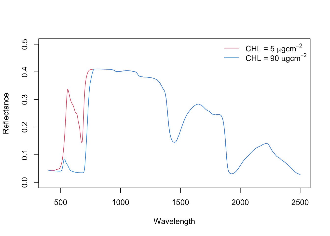

Note

Increasing chlorophyll content causes a) absorption in blue and red spectrum and b) red-shift of red-edge (to the right).

PROSAIL

PROSAIL is a fusion of PROSPECT (leaf reflectance and transmittance) and SAIL (plant canopy reflectance). Thus, the model simulates canopy reflectance based on leaf biochemical and structural parameters as well as canopy and observation geometry. PROSAIL been used for the last thirty years to simulate the spectral and directional reflectance of plant canopies in the solar domain. It links the spectral dimension of the reflectance, which is mainly related to the biochemical content of the leaves, to the directional dimension, which is mainly related to the architecture of the canopy (Jacquemoud et al., 2009).

?PRO4SAIL

The PRO4SAIL function of the prosail package runs the PROSAIL model. Check out the help pages for a description of the function arguments and model parameters. Here is an example of selected parameters:

Model	Parameter	Description
PROSPECT	N	Leaf structure parameter
	CHL	Cholorophyll a + b content
	EWT	Equivalent water thickness
	ANT	Anthocyanin content
	BROWN	Brown pigments content
	LMA	Leaf Mass per Area
SAIL	lai	Leaf area index
	TypeLidf	Leaf inclination distribution function
	LIDFa	if TypeLidf = 1, controls the average leaf slope if TypeLidf = 2, controls the average leaf angle
	LIDFb	if TypeLidf = 1, controls the distribution’s bimodality if TypeLidf = 2, unused
	q	Hot spot parameter
	tts	Solar zenith angle
	tto	Viewing zenith angle
	psi	Azimuth Sun / Observer
	rsoil	Soil reflectance

The PRO4SAIL function requires you to define the leaf properties (Input_PROSPECT), soil reflectance (predefined for wet and dry soil), and canopy parameters. The example below, defines the leaf parameters and uses a reflectance profile from a wet soil.

# define input variables for PROSPECT. 
Input_PROSPECT = data.frame('CHL' = 40, 'CAR' = 8, 'ANT' = 0.0, 
                            'EWT' = 0.01, 'N' = 1.5)

# wavelength
wvl <- SpecPROSPECT_FullRange$lambda 

# soil reflectance
rsoil <- SpecSOIL$Wet_Soil 

# run PROSAIL with 4SAIL
Ref_4SAIL <- prosail::PRO4SAIL(Input_PROSPECT = Input_PROSPECT, 
                      TypeLidf = 1, LIDFa = -0.35, LIDFb = -0.15,
                      lai = 5, q = 0.01, tts = 30, tto = 10, psi = 0, 
                      rsoil = rsoil)

PRO4SAIL returns a list containing different versions of reflectance factors. In the context of satellite measurements, we are interested in the bi-directional reflectance factor. So, we extract rsot and pair it with wavelength in a new data frame (here called bf).

• rddt: bi-hemispherical reflectance factor
• rsdt: directional-hemispherical reflectance factor for solar incident flux
• rdot: hemispherical-directional reflectance factor in viewing direction
• rsot: bi-directional reflectance factor
• fcover: Fraction of green Vegetation Cover (= 1 - beam transmittance in the target-view path)
• abs_dir: canopy absorptance for direct solar incident flux
• abs_hem: canopy absorptance for hemispherical diffuse incident flux
• rsdstar: contribution of direct solar incident flux to albedo
• rddstar: contribution of hemispherical diffuse incident flux to albedo

bf <- data.frame(wvl = wvl, refl = Ref_4SAIL$rsot)

plot(refl ~ wvl, data=bf, type='l')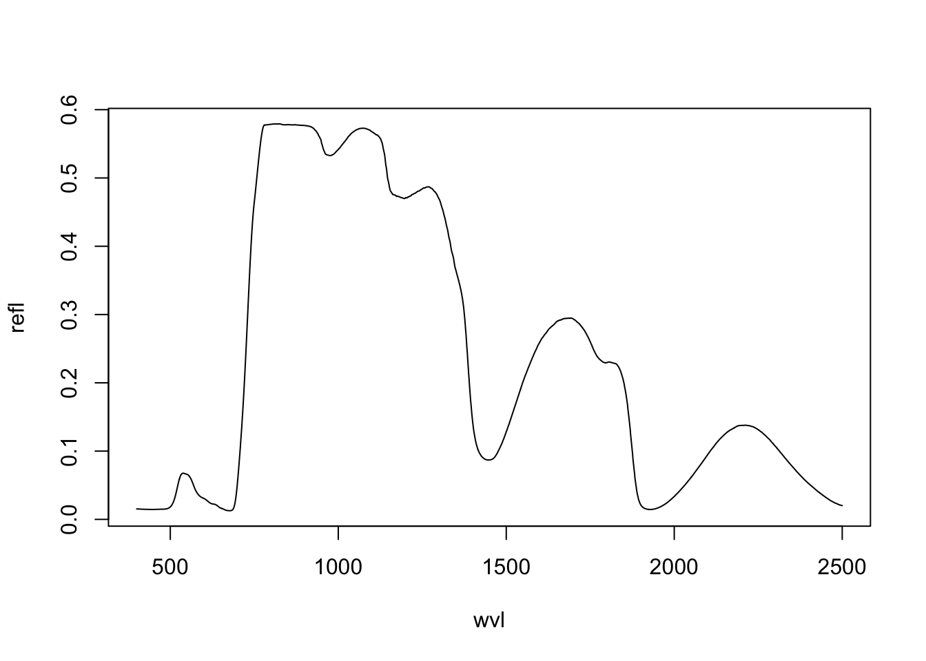

To test a range of different parameters, you need to run the PRO4SAIL function multiple times. For example, if you we want to test the effect of LAI on reflectance values, you can simulate the associated spectra by repeatedly calling PRO4SAIL and changing the input argument each time. This is quite cumbersome. So, for the purpose of this exercise, I created two convenience functions: 1) PRO4SAIL_batch and 2) PRO4SAIL_plot. To use the two functions in your assignment, you need to include (copy/paste) them into your markdown documents.

PRO4SAIL_batch <- function(...) {
  
  arg <- list(...)
  
  Input_PROSPECT <- data.frame('CHL' = 40, 'CAR' = 8, 'ANT' = 0.0, 
                            'EWT' = 0.01, 'LMA' = 0.009, 'N' = 1.5)
  
  varname <- names(arg)[1]
  values <- arg[[1]]
  
  wvl <- SpecPROSPECT_FullRange$lambda # wavelength
  
  result <- data.frame()
  for (val in values) {
    l <- list(Input_PROSPECT=Input_PROSPECT, var=val, TypeLidf=1,
              LIDFa=-0.35, LIDFb=-0.15, rsoil = SpecSOIL$Wet_Soil)
    names(l)[2] <- varname
    tmp <- data.frame(wvl = wvl, refl = do.call(prosail::PRO4SAIL, l)$rsot)
    if (!all(is.na(tmp$refl))) {
      tmp[, varname] <- val
      result <- rbind(result, tmp)
    }
  }
  return(result)
}

PRO4SAIL_plot <- function(spectra, ylim=c(0, 0.5)) {
  
  require(RColorBrewer)
  
  varname <- names(spectra)[3]
  values <- sort(unique(spectra[, 3]))
  colours <- brewer.pal(length(values), 'Spectral')
  
  for (i in seq_along(values)) {
    if (i == 1) {
      plot(spectra$wvl[spectra[, varname] == values[i]], spectra$refl[spectra[, varname] == values[i]], 
           ylim = ylim, col = colours[i], type='l', xlab="Wavelength [nm]",
           ylab = "Reflectance")
    } else {
      lines(spectra$wvl[spectra[, varname] == values[i]], 
                        spectra$refl[spectra[, varname] == values[i]], col = colours[i])
    }
  }
  
  labels <- paste(varname, "=", values)
  legend('topright', legend=labels, col=colours, lty=1, bty='n')
}

LAI

With PRO4SAIL_batch you can simulate bi-directional reflectance by changing a single SAIL parameter. For example, below we simulate reflectance LAI values 1 to 6. If you want to simulate the reflectance for a different parameter, just change the argument name and values in the function call.

spectra.lai <- PRO4SAIL_batch(lai=1:6)

With PRO4SAIL_plot you can visualize the output.

PRO4SAIL_plot(spectra.lai, ylim=c(0, 0.5))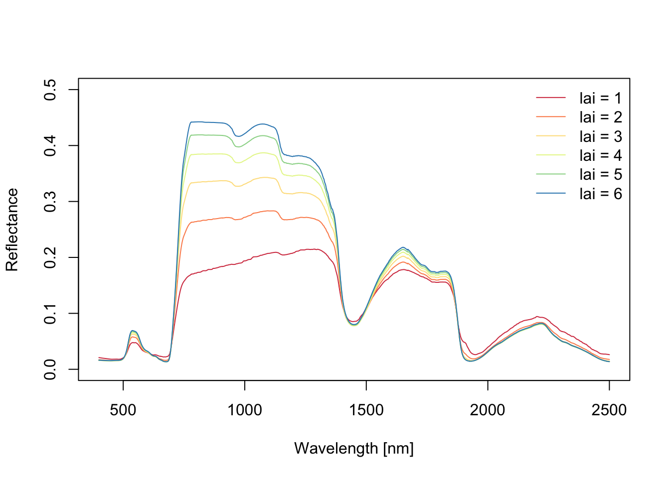

Note

Increasing LAI causes: a) increasing NIR, b) decreasing reflectance in red, and c) comparably small impact on shortwave-infrared.

Féret, J.-B., de Boissieu, F., 2024. Prosail: PROSAIL leaf and canopy radiative transfer model and inversion routines.

Féret, J.B., Gitelson, A.A., Noble, S.D., Jacquemoud, S., 2017. PROSPECT-d: Towards modeling leaf optical properties through a complete lifecycle. Remote Sensing of Environment 193, 204–215. https://doi.org/10.1016/j.rse.2017.03.004

Jacquemoud, S., Baret, F., 1990. Prospect - a model of leaf optical-properties spectra. Remote Sensing of Environment 34, 75–91. https://doi.org/10.1016/0034-4257(90)90100-Z

Jacquemoud, S., Verhoef, W., Baret, F., Bacour, C., Zarco-Tejada, P.J., Asner, G.P., François, C., Ustin, S.L., 2009. PROSPECT+SAIL models: A review of use for vegetation characterization. Remote Sensing of Environment 113, S56–S66. https://doi.org/10.1016/j.rse.2008.01.026